Deep Boltzmann Machine in THRML
Personal context
Since many months ago, I have been obsessed with a specific anomaly related to nuclear superradiance. I became concerned with the problem of accelerating the speed of parameter scan. This concern led me to the problem of constructing simulation for complex quantum systems.
What immediately came to mind was Feymann’s 1981 paper, in which he called for the construction of quantum computers as universal quantum simulators (Sec. 4). I consulted a few friends working on quantum computers. From them I drew an unanimous agreement: until fault-tolerant quantum computing becomes available, it would be much more productive to look to NN-based approaches.
It turns out there is a fascinating universe of research behind NN-based physics simulation. Neural quantum states (NQS) captures this body of research nicely, and this is an informative survey.
Meanwhile, Extropic announced its custom ASIC for probabilistic computing and a library that simulates their chip’s capability called THRML. Custom ASIC for energy-efficient ML has a special place in my heart, as I struggled with it during my PhD research and my work at Lightmatter 2019-21. I took at look at Extropic’s paper and decided to get my hands dirty with THRML and build a probabilistic model trained in Variational Monte Carlo (VMC) for a simple quantum system.
This two-part series captures what I learned along the way and some of my thoughts.
Energy-based model on a high level
Extropic’s chip works with energy-based models (EBM). I was not familiar with this family of models before, so I took the opportunity to give it a first-principle stare.
A side-note: in 2025, LLMs have become so good, given a problem X, I could ask a hundred questions about X in a row across multiple vendor models as my tutors to “impedance-match”: drill up and down depth-first until I bridge the gap between the frontier of my current knowledge and the prerequisite of X. Then I get to grasp X natively. These tutors would never get tired and that makes me sympathize with my younger self and the generations of people since the dawn of men who did not have access to this technology. Uncountably many sparks of curiosity were extinguished and people turned to other fields that were not necessarily their first pick for interest or impact.
Back to EBM. The motivating problem on a high level:
Given observations of a real world phenomena X that generates a data distribution \(P_D\), we wish to construct a mathematical machine that learns to generate samples as close to \(P_D\) as possible. Such a machine would be our simulator of phenomena X.
Sometimes it’s expensive or inconvenient to draw many samples from X in the real world. With a simulator at hand, we get to draw as many samples as our compute budget allows. Better yet, if the simulator can be primed by different parameters that characterize X, we get to study how X behaves in different regions of the parameter space: we get to perform parameter scan in computers instead of in lab or nature. This could accelerate the speed of discovery e.g. our simulator predicts X behaves in some desirable ways under such and such region in the parameter space; let’s test the prediction by running a costly experiment.
Algorithmically:
- Given \(P_D\), construct a simulator model parametrized by \(\theta\). Initialize \(\theta\) in some ways. The model generates samples from \(P_{\theta}\).
- Construct a measure of how similar \(P_{\theta}\) is from \(P_D\). We call this the loss function \(\mathcal{L}\), and a useful one here is the KL divergence. So $\mathcal{L} = D_{KL}(P_D || P_{\theta})$
- Compute the gradient of $\mathcal{L}$ with respect to $\theta$, or $\nabla_{\theta} \mathcal{L}$.
- Run backprop: $\theta \leftarrow \theta - \eta \cdot \nabla_{\theta} \mathcal{L}$, where $\eta$ is the learning rate.
- Repeat the above steps until convergence e.g. $\mathcal{L}$ plateaus or becomes sufficiently small.
Now, what inside this model? The EBM idea took a page from Boltzmann distribution and defined:
\[P_{\theta}(X) \propto e^{-E_{\theta}(X)}\]This says: “according to the model, the probability of the system under simulation occupying a particular state $X$ is proportional to expontential minus $E_{\theta}(X)$, where $E_{\theta}(X)$ is an energy function derived from the model.” In this expression, we observe that lowering the energy increases the probability. This reflects the physics intuition that systems prefer to occupy lower energy states.
For example, if we train a model to learn the ground state or some specific excited state of the 1-D particle in a box problem, we get to ask the model “how probable is the particle found in a specific location $x$ inside the box?” The model calculates $e^{-E_{\theta}(X)}$ and tells you the probability is proportional to that value.
But you protest and say you want the actual probability. Denote the state space as $\Omega$, then:
\[P_{\theta}(X) = \frac {e^{-E_{\theta}(X)}}{Z} = \frac {e^{-E_{\theta}(X)}}{\int_{\Omega} e^{-E_{\theta}(X')}dX'} \;\;or\;\; \frac {e^{-E_{\theta}(X)}}{\sum_{i \in \Omega} e^{-E_{\theta}(X_i)}}\]depending if the state space is continuous or discrete. Obtaining $Z$ is easy if $\Omega$ is small: you enumerate the entire space and compute the integral or summation. You get into trouble when $\Omega$ is large or infinite (read: the system can be in infinitely countable amount of possible states). This is the case for most problems of real world interest.
So now, we have two problems at hand:
- What does the model look like? And $E_{\theta}(X)$?
- What do we do if $Z$ is not attainable?
What does the model look like? And $E_{\theta}(X)$?
Here we have a fork in the road: MLP models or probabilistic models.
MLP (multilayer perceptron) typically defines a model where the input passes through a series of layer, each performing a matrix-multiply on its input, followed by a nonlinear activation. We call the output coming out of the final layer as logits. Invert the sign of logits and we get $E_{\theta}(X)$.
A probabilistic model typically consist of one visible layer and one or multiple hidden layers, each containing a number of nodes. Nodes across different layers are connected by the model parameters. Here’s the key difference from MLP: these nodes are random variables; they don’t relate deterministically to each other by matrix-multiply with $\theta$, instead their probability distributions conditioned on each other are defined over $\theta$. For example: denote the visible layer nodes as $\mathbf{v}$, a hidden layer connected to it as $\mathbf{h}$, and use only spin nodes e.g. every node’s range is $[0,1]$. Then we might write:
\[P(\mathbf{v_i}=1 \,|\, \mathbf{h}) = \sigma \left( b_i + \sum_{<i,j>}W_{i,j}\mathbf{h}_j \right)\]where $<i,j>$ runs through all the hidden layer nodes that are connected with $\mathbf{v}_i$ in our model architecture. $\sigma, b, W$ refer to our usual suspect: activation function, bias, and weight.
Finally, the energy $E_{\theta}(X)$ of a probabilistic model with nodes $\mathbf{s}$ (including visible and hidden) is typically defined as:
\[E_{\theta=\{b,W\}}(X=\mathbf{s}) = -\left( \sum b_i \mathbf{s}_i + \sum_{<i,j>} W_{ij} \mathbf{s}_i \mathbf{s}_j \right)\]In comparison:
- in MLP, you take the activations $h$ from layer $i-1$ and run it through $\sigma \left( b + W_{} h_{} \right)$ to get the activations of layer $i$
- in probabilistic computing models, you take the “activation samples” $h$ from layer $i-1$ and run it through $\sigma \left( b + W_{} h_{} \right)$ to get the Bernoulli probabilities that the nodes at layer $i$ would take value 1. You still need to sample from these distributions to get “activation samples” for the nodes at layer $i$.
What do we do if $Z$ is not attainable?
In other words, if we know a probability distribution $P = Z^{-1}f(X)$ without being able to normalize it to get $Z$, how do we generate samples of random variable $X$ from $P$? We must be able to do this, otherwise we can’t draw any samples from our trained probabilistic model which makes our effort pointless.
The key idea is that if even if we don’t know $Z$, given two candidate samples $X_1$ and $X_2$ at hand, we can know for sure $P(X_1) / P(X_2)$ because the $Z$’s cancel out. In other words we get to know their relative likelihood, $X_1$ over $X_2$.
So, given a trained model with parameter $\theta$, we can construct a process like the following to draw samples that are practically good from the model distribution $P_{\theta}$:
- Make an initial guess and produce a candidate sample $X_0$ (a particular state in $\Omega$). Set the visible layer nodes to this sample. This is where we start. At this point we have no idea how probable this sample is with respect to $P_{\theta}$. For example, if $P_{\theta}$ happens to be normal distribution $\mathcal{N}(0,1)$, $\Omega = \mathbb{R}$, and our initial guess is the number 7.19. This number is more than 7 standard deviations aways from mean and its $P_{\theta} \approx 3 \times 10^{-13}$, which means it’s extremely unlikely that our initial guess is in any practical sample batch drawn from this model.
- Propose a perturbation step $\Delta \in \Omega$, which we use to nudge the $X_0$ into $X_0 + \Delta$.
- Compute $P(X_0 + \Delta)/P(X_0) \rightarrow a$, where $a \in [0,1]$.
- Construct a Bernoulli distribution (rigged coin) with $a$: $Bernoulli(a)$
- Draw one sample from $Bernoulli(a)$
- if the sample is 1, we set $X_1$ to $X_0 + \Delta$ i.e. we make the jump.
- if the sample is 0, we set $X_1$ to $X_0$ i.e. we don’t jump.
- Repeat the above steps to generate $X_2, X_3, …$
After sufficient samples (called “warmup”), we will have jumped into a sufficiently balanced state where the samples are practically useful. Then, we continue the above steps to draw the samples we need.
The above is a general description of the Markov Chain Monte Carlo (MCMC) family of algorithms, among which Gibbs sampling is useful when $X$ is high dimensional.
Putting things together: training a Deep Boltzmann Machine
A Deep Boltzmann Machine (DBM) contains one visible layer and more than one hidden layer. Like Restricted Boltzmann Machine (RBM), nodes in the same layer don’t connect among themselves. Nodes connect to nearby layers.
Say we have a DBM with spin nodes only:
[ visible ($v$) ↔ hidden 1 ($h_1$) ↔ hidden 2 ($h_2$) ]
We want to train the model to learn a data distribution $P_D$, for which we have training samples $D$. After training, we want to generate more samples from the model i.e. inference.
We define loss as $\mathcal{L} = D_{KL}(P_D || P_{\theta})$, which upon throwing away terms unrelated to $\theta$ we rewrite loss as \(\mathcal{L} = - \mathbb{E}_{x \sim P_D}[log\,P_{\theta}(x)]\). This reads as “for the samples drawn from from data distribution, how unlikely is the model producing them”? We want to minimize this.
With this loss, its gradient is \(\nabla_{\theta}\mathcal{L} = \mathbb{E}_{x \sim P_{D}} \left[ \nabla_\theta E_\theta(x) \right] - \mathbb{E}_{x \sim P_{\theta}} \left[ \nabla_\theta E_\theta(x) \right]\). We are skipping the derivation here. We observe the gradient contains two expected values, one with samples drawn from $P_D$, the other with samples drawn from $P_{\theta}$.
We follow this training procedure reflecting what’s used in THRML:
- Recognize we have three important conditional distributions in this model: \(P(v=1\,\mid h_1)\), \(P(h_1=1\, \mid v,h_2)\), \(P(h_2=1\, \mid h_1)\). Notice $v$ does not connect to $h_2$ and how this is reflected in the distributions. Each of these distributions are parametrized in the form of $\sigma \left( b + W_{} h_{} \right)$. The collection of all ${b,W}$ forms the model parameter $\theta$.
- Initialize $\theta$. Initialize values at $h_1$ and $h_2$.
- Perform “positive phase” to compute the first expected value \(\mathbb{E}_{x \sim P_{D}} \left[ \nabla_\theta E_\theta(x) \right]\) (note: this is different from the mean-field approach used by the inventor of DBM in Salakhutdinov & Hinton 2009):
- Take samples $d \in D$ and set $v$ to $d$ i.e. “feeding” the model with training data from the visible layer. This step is also called “clamping” the visible nodes.
- Compute $P(h_1=1\, \mid v,h_2)$ and $P(h_2=1\, \mid h_1)$. They are concrete values.
- Perform Gibbs sampling to update $h_1$ and $h_2$. After the warmup iterations, draw samples of $h_1, h_2$, which together with $d$ are treated as samples drawn from $P_D$.
- Compute energies $E_{\theta}$ with samples of $d, h_1, h_2$.
- Compute their gradients $\nabla_\theta E_\theta(x)$.
- Compute their mean, which gives us \(\mathbb{E}_{x \sim P_{D}} \left[ \nabla_\theta E_\theta(x) \right]\).
- Perform “negative phase” to compute the second expected value \(\mathbb{E}_{x \sim P_{\theta}} \left[\nabla_\theta E_\theta(x)\right]\):
- Set the nodes $v, h_1, h_2$ to an initiate set of values.
- Compute $P(v = 1 \mid h_1)$, $P(h_1=1\, \mid v,h_2)$ and $P(h_2=1\, \mid h_1)$.
- Perform Gibbs sampling to update $v, h_1, h_2$. After the warmup iterations, draw samples of $v, h_1, h_2$, which are treated as samples drawn from $P_\theta$.
- Compute energies $E_{\theta}$ with these samples.
- Compute their gradients $\nabla_\theta E_\theta(x)$.
- Compute their mean, which gives us $E_{x \sim P_\theta} [ \nabla_\theta E_\theta(x) ]$.
- Take the two expected values and assemble $\nabla_{\theta}\mathcal{L}$.
- Perform backprop $\theta \leftarrow \theta - \eta \cdot \nabla_{\theta} \mathcal{L}$.
- Repeat step 3-6 until convergence.
Learning a bi-modal univariate Gaussian
I trained a DBM to learn a bi-modal univariate Gaussian. You can find the code here.
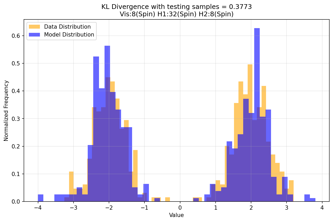
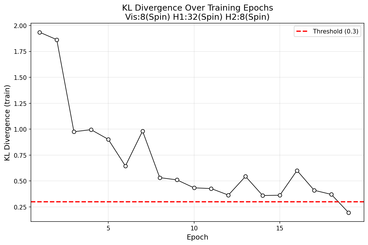
The model has 2 hidden layers and contains only spin nodes. Floats drawn from $P_D$ are quantized into binary representation for clamping the visible nodes during positive phase. For computing $D_{KL}$, samples from $P_{\theta}$ are de-quantized and compared against samples from $P_D$. Below is a plot of $D_{KL}$ over epoch.
Below is the histogram of samples drawn from $P_D$ overlaid with the histogram of samples drawn from $P_{\theta}$ after training ends.