Variational Monte Carlo in THRML & thoughts on Extropic
Ab-initio simulation of quantum systems
Ab-initio simulation, or first-principle simulation, learns the behavior of phenomenon X given only the mathematical rules that govern X. It does not need observational data of X in the real world.
This is particularly valuable in the engineering of quantum systems, due to at least the following reasons that can make experiment slow and costly:
- Quantum states cannot be cloned.
- Measurement collapses states.
With ab-initio simulation, given the definition of a quantum system of interest, we get to produce a simulated version of its wavefunction $\psi(X)$ as a function of system state $X$. With this wavefunction at hand, we can:
- apply different operators and produce simulated observables.
- explore the behavior of wavefunction given different system definition i.e. we can sweep the system parameter space at the speed of how fast we can construct simulations, not how fast we can run experiments.
Most interestingly, we can start asking the inverse design question: given ABC desirable properties of the resulting wavefunction, what does the quantum system look like? We can answer the question at the speed of what our compute budget allows.
Variational Monte Carlo
Variational Monte Carlo (VMC) is an ab-initio method primarily for simulating quantum systems at their ground states. Below is walkthrough of the method in simple language.
“Variational” in VMC means to find a solution to a problem by (1) starting with a guess for what the solution looks like, parameterized by $\theta$, which is initialized in some way (2) searching in the $\theta$ space by varying $\theta$ until we fine the solution.
The guess for what the solution looks like is called the ansatz.
In the context of finding the wavefunction given the definition of a quantum system, the system definition typically takes the form of a Hamiltonian, and the mathematical rules are dictated by the Schrödinger equation. What do these mean?
A detour into quantum mechanics
In classical physics, people are concerned about what is: they assume the world exists and evolves independent of observations made on them. In quantum physics, a new world view born ~100 years ago, specifically with the Copenhagen interpretation, people are concerned about what can be observed. We cannot understand anything about the world unless we make observations.
The Schrödinger equation is a mathematical tool to describe how a system state evolves before observations are made on the system. It is a useful tool because the predictions it makes about the probabilities of possible observational outcomes match experimental data with extraordinary accuracy.
The wavefunction $\Psi(X,t)$ encodes both the superposition of all possible system states $X$ and the evolution of this superposition in time $t$. If we are interested in an observable $o$, we take the corresponding operator $\hat{o}$ and make it act on the wavefunction: $\hat{o}\Psi$. A particular operator of interest is the Hamiltonian $\hat{H}$, the operator for the total energy of the system. We use it to write down the Schrödinger equation:
\[\hat{H}\Psi = E \Psi\]Given a closed system, we have energy conservation, meaning energy $E$ is constant. This allows us to decompose the wavefunction into a function of time, $\phi$, and a function independent of time, $\psi$: $\Psi(X,t) = \psi(X) \cdot \phi(t)$. We can then write down the same equation in time-independent form:
\[\hat{H}\psi = E \psi\]This equation is really useful. Given a system definition, we can apply the applicable physical laws to write down the Hamiltonian $\hat{H}$. We can then try to solve this equation to obtain $E_n$, the nth allowed energies of the system with arbitrary n, and the corresponding stable stationary state $\psi_n$.
For example, we can use this equation to study the only electron in a hydrogen atom. In this case, $\hat{H}$ contains the kinetic energy operator ($-\frac{\hbar^2}{2\mu}\nabla^2$, where $\mu$ is the reduced mass of electron-proton, and $\hbar$ is the plank constant divided by $2\pi$) and the potential energy operator ($-\frac{e^2}{4\pi\varepsilon_0}\,\frac{1}{r}$, which is just the static Coulomb potential). The state of the electron is described by the vector $\mathbf{r}$ pointing from the nucleus to the electron (there is only one electron in the system, so we ignore spins). The equation goes:
\[\left[ -\frac{\hbar^2}{2\mu}\nabla^2 \;-\; \frac{e^2}{4\pi\varepsilon_0}\,\frac{1}{r} \right]\psi(\mathbf{r}) = E\,\psi(\mathbf{r})\]If we solve this equation for the lowest possible $E$, we will find it to be $-13.6\;\text{eV}$, exactly the ground state energy of the hydrogen electron.
VMC in math
It turns out we cannot analytically solve the Schrödinger equation for systems even only slightly more complex than hydrogen. We need numerical methods to approximate the solution. VMC is one such method., at least dating back to the McMillan 1965 paper.
The general idea of VMC is as follows. Create a mathematical machine parametrized by $\theta$. This machine takes a system state $X$ and returns its unnormalized wavefunction $\psi_{\theta}(X)$. Then, define two terms: local energy $E_{loc}(X)$ (the system energy at state $X$) and the expected value of energy $\langle E \rangle$:
\[E_{\mathrm{loc}}(X) = \frac{(\hat{H}\psi_\theta(X))}{\psi_\theta(X)}\] \[\langle E \rangle = \frac{\langle \psi_{\theta}| \hat{H} | \psi_{\theta}\rangle}{\langle \psi_{\theta}| \psi_{\theta}\rangle} = \mathbb{E}_{X \sim |\psi_\theta|^2}\!\left[\, E_{\mathrm{loc}}(X) \,\right].\]VMC finds the ground state energy $E_0$ of the system described by $\hat{H}$ by searching in $\theta$ space until $\langle E \rangle$ is minimized. The resulting value is $E_0$.
This leads us to three major troubles:
- Given a Hamiltonian, what ansatz for $\psi_{\theta}(X)$ should we start with? What does the solution look like for any nontrivial quantum system?
- How do we efficiently search in $\theta$ space?
- How to draw $X \sim |\psi_{\theta}|^2$?
VMC with backprop: using a neural network as the wavefunction ansatz
Possibly the first paper that uses a neural network as the wavefunction ansatz is Carleo & Troyer 2016. Not just any neural network. They used RBMs. Why? From the perspective of the three troubles listed earlier:
- Neural networks have proven to be expressive ansatz. By 2016 neural networks have break records in both image recognition and language modeling. It makes sense to apply them to physical phenomena. Not only are they expressive, they are also flexible: there exist a wide variety of neural network architectures with different complexities and properties, and for each architecture we can tune their hyperparameters for our need.
- The training procedure of neural networks explores the $\theta$ space. There exists a wide variety of techniques and heuristics for training.
- RBM represents $X$ as explicit random variables at its visible layer. We can draw $X \sim |\psi_{\theta}|^2$ by running RBM in the negative phase.
The general approach works as follows:
- Given a system description and its Hamiltonian $\hat{H}$, design an RBM, parametrized by $\theta$, whose visible layer corresponds to the system state $X$. Initialize $\theta$. We are ready to train.
- Run MCMC until the Markov Chain is sufficiently balanced. Draw $M$ samples of $X$ from the model distribution $P_{\theta} = |\psi_{\theta}|^2$.
- Compute loss function \(\mathcal{L} = \langle E \rangle = \mathbb{E}_{X \sim P_{\theta}(X)}\!\left[\, E_{\mathrm{loc}}(X) \,\right] = \frac{1}{M}\sum_{i}E_{loc}(X_i)\) using the samples.
- Compute the loss gradient $\nabla_{\theta} \mathcal{L}$.
- Update parameter $\theta \leftarrow \theta - \eta \cdot \nabla_{\theta} \mathcal{L}$.
- Repeat step 2-5 until convergence.
The VMC loss gradient has a classic form:
\[\nabla_{\theta}\mathcal{L} = 2\cdot \frac{1}{M}\sum_{i} \,(E_{loc}(X_i)-\langle E \rangle) \cdot \nabla_{\theta} \,log | \psi_{\theta}(X_i) |\]When applying this approach to a concrete problem, we need to derive a few things first:
- Derive $|\psi_{\theta}(X)|$. Define an RBM architecture, which automatically gives us its energy expression $E_{\theta}(X)$. Because for RBMs, $P_{\theta}(X) \propto e^{-E_{\theta}(X)}$, and $P(X) = |\psi_{\theta}(X)|^2$, we can derive $|\psi_{\theta}(X)|$. This is needed for $\nabla_{\theta} \,log | \psi_{\theta}(X_i) |$ in the gradient expression. Using modern software package, we can typically perform $\nabla_{\theta}$ by auto-differentiation.
- Derive $E_{loc}(X)$. Write down $\hat{H}$, which allows us to derive $E_{loc}(X)$. This may involve $|\psi_{\theta}(X)|$.
We are now ready to apply this approach to a simple quantum problem.
The 1-D TFIM problem
The 1-D Transverse-Field Ising Model problem is a simple model with analytical solution for its ground state energy. We can compare it against the value found by RBM+VMC.
Imagine a number of particles arranged in a 1-D chain along the Y-axis. Each particle (called a site) has two possible spin states along the Z direction: up or down. Each particle is coupled to its neighbors in a way that either prefers a pair of neighboring particles to have the same or opposite spin. This coupling is captured by the strength $J$. Now apply a magnetic field in the transverse direction X (technically, any direction on the X-Y plane is transverse to Z, but we choose X for simplicity). This magnetic field has the effect of creating coherent oscillations of the particle’s spin. The strength of this transverse field is $\Gamma$. Here we use $J \ge 0$ (ferromagnetic) and $\Gamma \ge 0$.
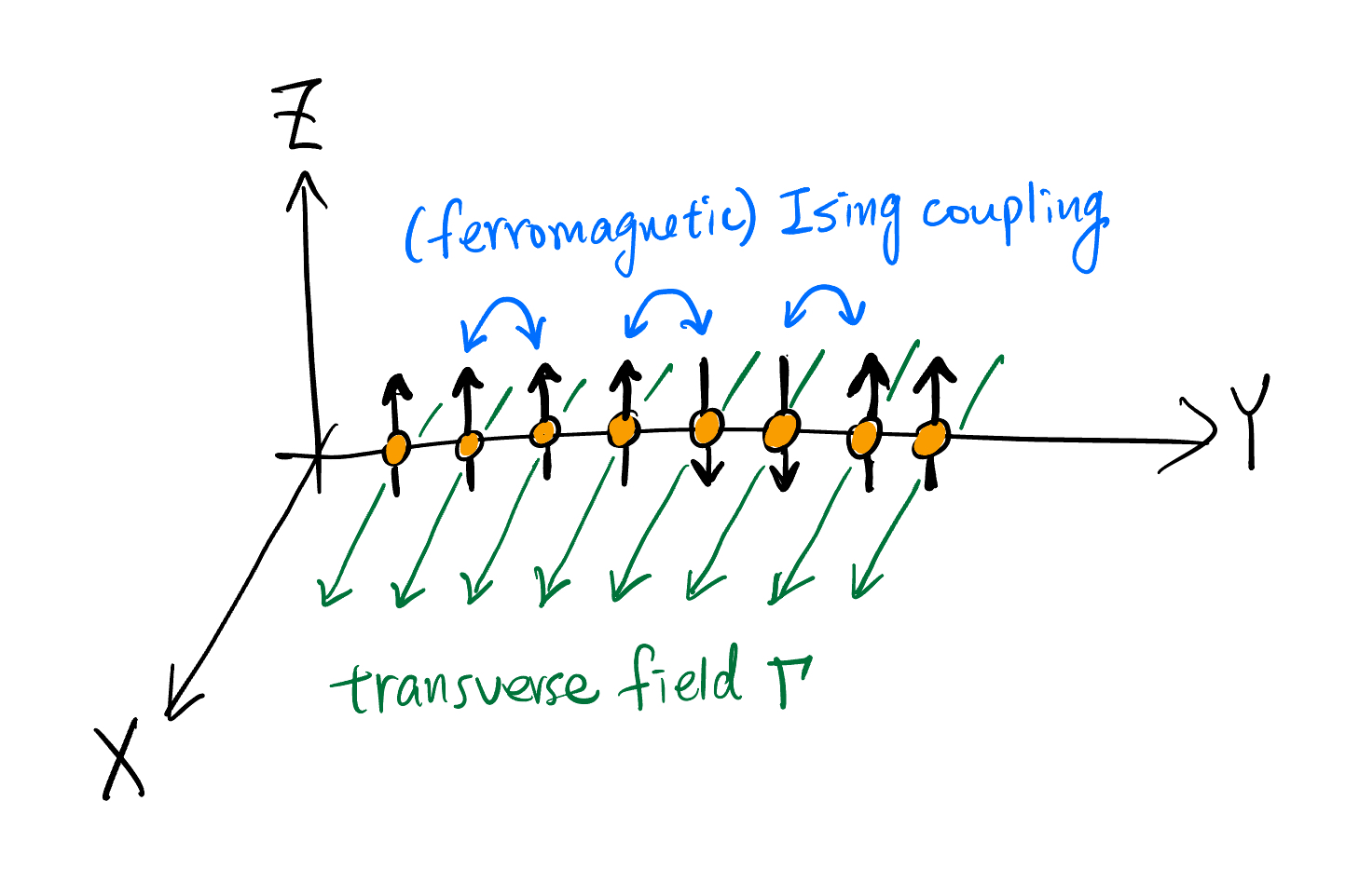
The Hamiltonian for 1-D TFIM is typically written as:
\[\hat{H} = -J\sum_i \hat{\sigma}^z_i \hat{\sigma}^z_{i+1} - \Gamma\sum_i \hat{\sigma}^x_i\]Let’s break it down. We can see the Hamiltonian expression involves two operators: $\hat{\sigma}^z_i$ and $\hat{\sigma}^x_i$. These are the Pauli matrices. $\hat{\sigma}^z_i$ measures the z-spin of a the $i^{\text{th}}$ particle. $\hat{\sigma}^x_i$ flips the z-spin of the $i^{\text{th}}$ particle.
Specifically, using the ket notation (a ket $\ket{}$ is just a particular wavefunction state; more precisely, a ket denotes a vector in the Hilbert space, where wavefunction lives):
\[\hat{\sigma}^z \ket{\uparrow} = +1 \ket{\uparrow}; \;\;\hat{\sigma}^z \ket{\downarrow} = -1 \ket{\downarrow}\]From these relations, we can see how $\hat{\sigma}^z_i \hat{\sigma}^z_{i+1}$ contribute to the total energy: if the spins of the $i^{\text{th}}$and $i+1^{\text{th}}$ particle are $\uparrow \uparrow$ or $\uparrow \uparrow$, the term yields +1, which contributes $-J$ to the total energy. If their spins are $\downarrow \uparrow$ or $\uparrow \downarrow$, the term contributes $+J$ to the total energy. With $J \ge 0$, this tells us the system favors aligned neighbors.
And the flipping in action:
\[\hat{\sigma}^x \ket{\uparrow} = \ket{\downarrow}; \;\;\hat{\sigma}^x \ket{\downarrow} = \ket{\uparrow}\]In fact, the effect of $-\Gamma \sigma^x$ in the Hamiltonian is to cause a particle to oscillate between the two spin states: $\ket{\Psi(t)} = \cos(\Gamma t)\,\ket{\uparrow} + i \sin(\Gamma t)\,\ket{\downarrow}$.
We are now two steps away from being ready to train an RBM with VMC for this problem: (1) derive $|\psi|$ (2) derive $E_{loc}$.
Find $|\psi(S)|$
We denote the state as \(S = \{s_i \in \{-1, +1\},\,i\in 1...N\}\), meaning we have $N$ particles in total, the spin state of each takes either -1 (down) or +1 (up).
We define a RBM model with exactly $N$ spin-nodes in the visible layer, one for each particle in the problem, and $M$ spin-nodes in the hidden layer. The state of the hidden layer is denoted as \(H = \{h_i \in \{-1, +1\},\,i\in 1...M\}\)
The RBM’s energy is then:
\[E_{\theta}(S,H) = -\beta \left( \sum_{i=1}^N a_i s_i + \sum_{j=1}^{M} b_j h_j + \sum_{<i,j>} w_{ij} s_i h_j \right)\]where $a_i, b_j$ are biases for each node in the visible and hidden layer, and $w_{ij}$ is the weight on the edge connecting visible node $s_i$ to hidden node $h_j$. $\beta$ is temperature, a hyperparameter for tuning the sharpness of $P_{\theta}$.
Because for RBMs, $P_{\theta}(X) \propto e^{-E_{\theta}(X)}$, and $P(X) = |\psi_{\theta}(X)|^2$, we have
\[\|\psi(S,H)\| \propto e^{-\frac{1}{2}E_{\theta}(S,H)}\]Then $|\psi(S)|$ is just marginalizing $|\psi(S,H)|$ over all possible states of $H$. We take advantage of RBM’s property that nodes in the same layer are independent to each other, so marginalization is done by doing the sums involving $h_j$ twice, once with $h_j=1$, once with $h_j=-1$. We skip the derivation here and write down $|\psi(S)|$ in log form:
\[log| \psi (s) | = \frac{1}{2} \left[ \beta\sum_i a_i s_i + \sum_j log \left[ 2\cosh \left(\beta (b_j + \sum_i W_{ij} s_i) \right) \right] \right] + const.\]Find $E_{loc}(S)$
Recall:
\[E_{\mathrm{loc}}(X) = \frac{(\hat{H}\psi_\theta(X))}{\psi_\theta(X)}\]Plug in the Hamiltonian, we’ll find (derivation skipped):
\[E_{loc}(s) = -J \sum s_i s_{i+1} - \Gamma \sum_i \frac{\psi(S^{(\sim i)})}{\psi(S)}\]where $\psi(s^{(\sim i)})$ is the wavefunction at state $S$ with the spin of the $i^{\text{th}}$ particle flipped in direction. The conventional notation for this is $\psi(s^{(i)})$, but to me it doesn’t really convey the flip. So I invented $\psi(s^{(\sim i)})$.
Now, with $|\psi(S)|$ and $E_{loc}(S)$ derived, we can proceed with training.
1-D TFIM in THRML
I constructed in THRML an RBM and trained it with VMC for the 1-D TFIM problem. You can find the code here.
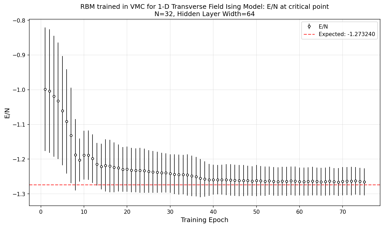
The model has $N=32$ in the visible layer, $M=64$ in the hidden layer. I am burning 20000 samples for warmup during Gibbs sampling, and taking 10000 samples for expected value calculation, 50 steps between consecutive samples.
Since the analytical solution for the ground state energy per site ($E/N$) is readily available, I plot the model’s predicted $E/N$ over training epoch, with standard deviation of $E/N$ shown as the half width of error bar, at the critical point condition $J = \Gamma = 1$:
Below is a p5.js animation of 20 states sampled from the trained RBM:
The analytical solution for ground state energy per site at the critical point is $-4/\pi \approx -1.27324$ (first solved possibly in Lieb, Schultz & Mattis 1961, later in Pfeuty 1970 in a more modern notation; Pfeuty used the operator $\hat{S}$ which is half of $\sigma$ with $\hbar$ set to 1).
At convergence, our model prediction is within 0.5% from the analytical solution.
Thoughts on Extropic’s strategy and the survivability function
First I want to credit this blog by Zach, from which I learned about the universe of works on pbits and Ising machines. I want to cut Extropic some slack about engineering novelty, as I believe success here depends more on timing (luck), execution, and steermanship.
As I gain clarity on the procedure of sampling EBMs, I begin to consider the architecture of Extropic’s chip and their PR strategy. I have a few thoughts:
- Fashion MNIST is a fairly small dataset. Evaluation results based on it constitute at most evidence toward Technology Readiness Level 4 (TRL 4; validation in lab environment). In my impression, most TRL 4 accomplishments, born in academic or corporate labs, are publicized in the form of academic papers, press release on niche professional channels, and announcements on the lab homepage. Few would catch the attention of mass media. On the other hand, Extropic seems to lean heavily into capturing the attention space on mass social media.
- It seems full connectivity between layers is not supported on the chip, despite THRML supporting it. I infer that software abstractions simulating full connectivity on top of sparsely connected nodes are offered and I wonder how performant they are. I do imagine sparsity being prevalent in many useful models, but higher generality at the hardware level seems wise because it broadens the algorithmic coverage of their offering.
- I do not have my hands on an Extropic chip. I imagine the THRML API is representative of the frontend of their stack, which may have one or more processors (RISC-V via SiFive?) configured with extra opcodes to program and access the pbits via FPGA as bridge (SoC could be too costly at this stage). If so, as seen in the THRML API, Extropic’s chip does not support continuous nodes. This matches what Extropic’s founder said on X that float is not supported. I wonder how expensive it would be to operate a software abstraction for continuous nodes based on the discrete pbits. When would continuous nodes be useful? For instance, I tried to build a DBM and train it with VMC to learn the wavefunction of a particle trapped in a 1-D potential well and predicts its ground state energy. The state of the particle is continuous, while THRML provides only spin & categorical nodes. I was going for accuracy against $\frac{1}{2} \omega$ ($\hbar=1$), so I didn’t consider the grid approach and tried both binary codes and gray codes for quantization. I ran into troubles with gradients, specifically second-order derivatives with respect to the continuous state variable. For sure, there exist other approaches for derivatives (e.g. finite difference) and quantization (e.g. grids), but I would imagine a chip supporting continuous nodes, at least in the form of performant software abstraction, opens up larger grounds of research and application opportunities.
I begin to speculate the strategic consideration behind these choices. Having struggled at early stage startups and made numerous mistakes, I understand the thrill of backfilling from a bright future prediction and the challenge of operating with unclear short-term demand, tremendous technical risks, and tremendous incumbent domination. So I refrain from judging from the outside.
That said, I want to assume that the team possesses certain Thielian secrets and has been acting with max rationality. With that assumption, I assume the ultimate objective of all their design choices and PR strategy is to argmax Extropic’s survivability until their secret manifests in reality. What can we infer about their secrets and their survivability function?
I think one big factor in their survivability function is that Extropic must continue to attract funding to pay for tape-outs to climb the TRL. How would they do it?
I think they need these two factors to work:
\[\text{(1) TAM of EBM paradigm} \times \text{(2) Extropic’s share of EBM compute}\]If (1) is small, there’s no win. If (1) is large but GPU gets really good for EBMs such that (2) is small, there’s still no win. Win in the sense of a 100x bagger as a venture-backed startup.
For (1), it should be incredibly difficult to engineer paradigm growth/shift as a startup. But, they couldn’t afford to just wait for the paradigm to take off either, because as a company they are default dead, unlike Nvidia being paid by the gaming market to drive down the cost curve of GPUs for many years prior to Nvidia’s discovery of the NN paradigm in ~2013. So Extropic needs to do what they can to grow (1) & (2), but to do so while conserving capital because many factors behind (1) are beyond Extropic’s control e.g. when AI company valuations price in energy as bottleneck. I think capital conservation can explain the design choices of not supporting full connectivity (which requires analog crossbar, which is area-expensive) and not supporting continuous nodes (which would require precise ADCs, which are also area-expensive).
A second order factor is the amount of creative researchers and product designers tinkering with EBMs. We don’t know when the EBM algorithm family could surpass transformers in language modeling and world modeling. New killer application scenarios may have to be discovered. Social media buzz, academic collaboration, hackathons etc are all useful for driving this knob, to funnel more people into this paradigm and bet on the wisdom of the crowd to find something to grow (1).
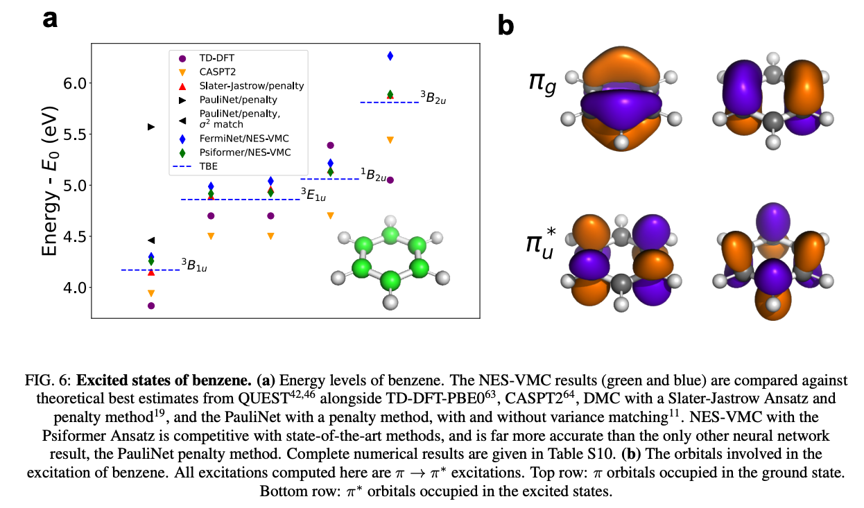
Yet another second order factor is to counterposition, which requires avoiding applications that run extremely well in the existing paradigm (largely deterministic models on GPU) for (2). This can also explain why floating point support is dropped, at least partially. Physics and quantum chemistry workloads work extremely well with the existing paradigm with no obvious ceiling in the near future e.g. see Pfau et. al. 2024 (Fig. 6 adapted below) where attention network ansatz gives competitive results against theoretical best estimates for the excited states of $\text{C}_6 \text{H}_6$, a medium-sized molecule!
Public attention maximization should contribute to recruiting, which is a second order factor for (2). But I am wary of this: social media hype at TRL 4 can generate mistrust for senior circuit design engineers. Among those I have known in person, they are fairly risk averse. Their spouses can be a dominant factor behind their career decision making. However aligned I am personally with the mission to climb the Kardashev scale, I cannot imagine the buzzword being associated with household economic stability in the eyes of their spouses. But I think the play here is to optimize distribution first, optimize product second.
In conclusion, the bottomline for Extropic looks something like: ship a tinker-ready platform early → optimize exposure to tinkerers (i.e. public attention is their oxygen) → do everything they can to speed up truth-seeking for the EBM paradigm → focus differentially on demand that favors their custom chip over GPUs → survive long enough until GPT-10 or Genie-7 turn out to be heavily reliant on sampling, which may be Extropic’s Thielian secret.