RTL exercises for qubit control

Special thanks to Ko-Wei Tseng, Justin Hou and Allen Chiu for inspirations.

Motivation

I have become fascinated by quantum computers, so I spent a month studying their various architectures and the underlying physics.

Some architectures require resonant driving with microwave AC pulses. Some others require optical laser pulses with detuning to perform the two-photon Raman transition. One thing in common is the stringent requirement on their control systems. Precise pulse-shaping is critical in minimizing noises in qubit state preparation, single-qubit / two-qubit gates, and state readout. Real-time feedback with <1 μs response time is critical for error correction. PID control to suppress drift in laser intensity, frequency, phase.

This is how FPGA comes into play. Wanting to get hands-on, and curious about where open source EDA tools stand, I built two exercises for myself:

1. A simple TX controller for JESD204B.
2. A simple pulse generator for DRAG and Wah-Wah.

Open source EDA tools

Previously at school and at work, I was used to VCS and ModelSim. For these exercises, I use open source tools:

• Verilator as RTL simulator;
• GTKWave as waveform viewer.

I wanted to write UVM-like testbench, which requires the use of SystemVerilog classes. However, Verilator has trouble with virtual interfaces, which are required for classes to access the actual interfaces of DUT. I saw an open issue and decided to decouple my exercises from this trouble. Simple, flat testbenches were written with UVM framework in mind - sequencer, driver, monitor and scoreboard.

Implementation notes

I follow particular best practices for synthesizable RTL. For example:

• I like to keep my sequential logic in always_ff blocks free of combinational logic.
• for flops, I like to declare flop_d and flop_q for the flop’s D pin and Q pin respectively, update q with d in the sequential blocks, and declare the combinational calculation for flop_d (1) with assign if it’s simple (2) with always_comb cases when it’s not.

I don’t like transitions sharply aligned with clock edges. I like to see propagation delays in my waves. As a result:

• I add #T_CQ to model the clock-to-Q delay whenever I do non-blocking assignments.
• I use clocking blocks to add skews when I drive signals in the testbench.

RTL exercise 1: JESD204B TX

High speed ADC/DACs are required for sending and receiving pulses to qubits across many QC architectures. I decided to write up a TX controller RTL for JESD204B, a high speed interface which commonly sits between high speed data converters and FPGAs.

Schematics

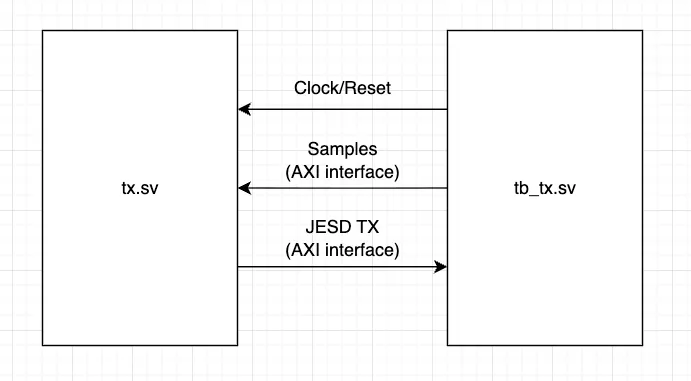
tx.sv implements a controller that sits between (1) the imaginary internal control system logic and (2) the JESD core IP, which controls the transport, link, and PHY layer of JESD204B interface.

Testbench tb_tx.sv provides clock and reset, mocks the internal control system logic that drives samples into tx.sv, and mocks the JESD core IP. Interface follows AXI handshake protocol.

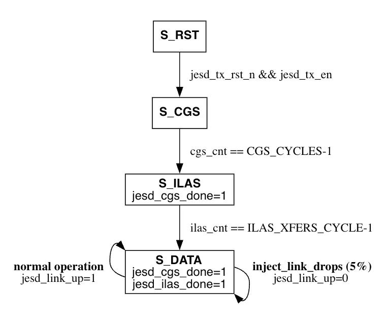
The state machine of the JESD core IP mock (reference for JESD link layer behavior), injecting link drops at 5% probability during DATA state:

Design

The design of tx is pretty simple. It sits between the sample-feeding interface of the internal control system logic on the upstream and the JESD core IP on the downstream, both following AXI handshake. To efficiently transmit data and relay backpressure, the data path features a skid buffer (skid_buffer.sv). In this exercise, upstream samples are zero-padded and passed down. tx monitors status flags from JESD core IP (jesd_cgs_done, jesd_ilas_done, jesd_link_up) and transmits data when the downstream is expecting data per these flags.

Result

To compile SystemVerilog sources into an executable; the resulting executable tb_sim can be found under the generated folder obj_dir :

verilator -Wall --sv --trace --binary tb_tx.sv tx.sv skid_buffer.sv --top-module tb_tx -o tb_sim

To run the executable and dump the waveform:

./obj_dir/tb_sim +VCD

To view the waveform:

GTKWave tb_tx.vcd

CLI message indicating test passing:

>./obj_dir/tb_sim +VCD
-----------------------------------------------------------
PASS: Completed simulation. expected_sample_queue is empty.
Matched samples = 501 (dut_ingested_samples=501)
-----------------------------------------------------------
- tb_tx.sv:347: Verilog $finish
- S i m u l a t i o n   R e p o r t: Verilator 5.042 2025-11-02
- Verilator: $finish at 7us; walltime 0.005 s; speed 1.642 ms/s
- Verilator: cpu 0.004 s on 1 threads; alloced 0 MB

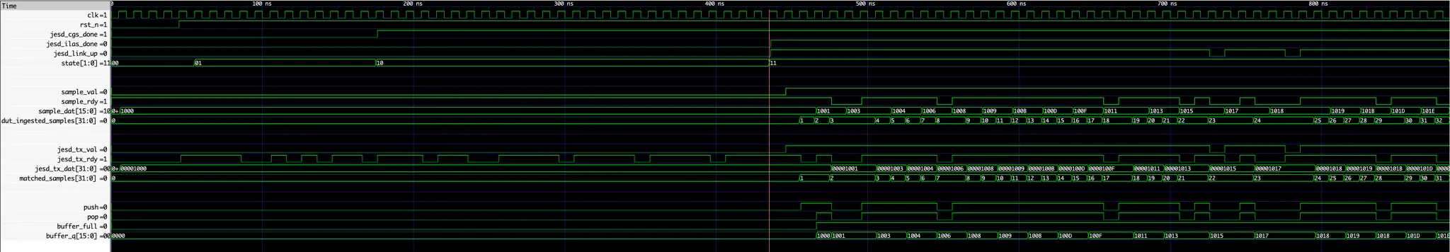
The resulting waveform, as viewed in GTKWave:

RTL exercise 2: Pulse Generator

I decided to write up a pulse generator that generates the in-phase and quadrature samples of parametrized pulse envelopes designed to suppress internal leakage through DRAG and external leakage through Wah-Wah.

Qubit control with pulse shaping

A pulse consists of a carrier wave oscillating within an envelope. The frequency of the carrier wave is set according to the architecture and the task. For example, to rotate a superconducting qubit with a specific $ω_{01}$ (5-7 GHz; in the microwave range), the frequency of the carrier wave is set to the same value.

The envelope determines the intensity and duration of the pulse. Intensity determines how fast the qubit state rotates through Rabi oscillation. Together with duration, they determine the actual amount of rotation performed.

Due to the sharp change in the time domain at the beginning and end of a pulse, a broad range of frequency components are introduced into the pulse’s spectrum. The goal of pulse shaping is to suppress unwanted frequency components, which are sources of noise.

DRAG pulse

DRAG pulse is designed to suppress internal leakage: the target qubit state drifting outside of \(\{\ket{0}, \ket{1}\}\) and into \(\ket{2}\), \(\ket{3}\) etc. Internal leakage into \(\ket{2}\) happens e.g. when the qubit in \(\ket{1}\) is driven by a non-negligible frequency component close to \(\omega_{12}\).

The DRAG (Derivative Removal by Adiabatic Gate) technique was proposed by Motzoi et. al. in 2009 in this paper. Limiting to a three-level system \(\{\ket{0}, \ket{1}, \ket{2}\}\), and denoting the in-phase and quadrature components as \(I(t)\) and \(Q(t)\) respectively, they found that setting \(Q(t) \propto \frac{dI(t)}{dt}\) can suppress leakage to \(\ket{2}\) to the first order of the pulse amplitude. Higher-order leakage suppression is possible but we limit this exercise to first-order DRAG.

In discrete time, using Gaussian for \(I[n]\), we have:

where:

in which \(\beta\) is a tunable parameter for DRAG.

Wah-Wah pulse

Wah-Wah pulse is designed to suppress external leakage: the states of neighboring qubits drifting outside of \(\{\ket{0}, \ket{1}\}\) and into \(\ket{2}\), \(\ket{3}\) etc. External leakage of qubit \(j\) in \(\ket{1}^j\) into \(\ket{2}^j\) happens when (1) there is a non-negligible frequency component close to \(\omega^j_{12}\) present in the pulse targeting qubit \(i\), and (2) qubit \(i\) and \(j\) are neighbors and share the same microwave line.

The Wah-Wah (Weak AnHarmonicity With Average Hamiltonian) technique was proposed by Schutjens et. al. in 2013 in this paper. Qubits sharing the same microwave line are set to different frequencies (\(\omega_{01}\)) but this can result in one’s \(\omega_{01}\) only slightly detuned from its neighbor’s \(\omega_{12}\) (leakage transition), as shown in the following diagram extracted from the 2013 paper:

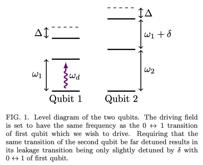
They found that by modulating the original \(I(t)\) (e.g. a Gaussian envelope) with a \([1 - A_m \cos{\omega_m (t-\mu)}]\) term, \(\mu\) being the same as that used in the Gaussian term, and \(Q(t)\) follows the DRAG technique, external leakage can be suppressed.

So we have in discrete time:

where:

in which \(\beta\), \(A_m\), \(\omega_m\) are tunable parameters for Wah-Wah.

Schematics

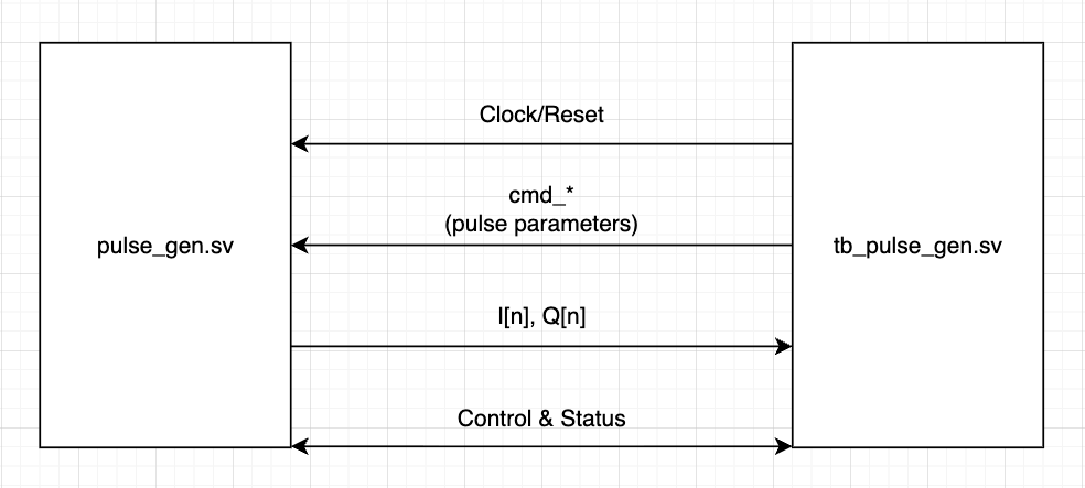
TB sets the pulse parameters and trigger pulse generation by asserting start.

The pulse generator module generates \(I[n]\) and \(Q[n]\) samples in a continuous stream, asserts busy when generating samples, and asserts out_last when the last sample of the current pulse is at the output.

The pulse generator would refuse to generate samples if the pulse parameters are erroneous: pulse sample length must be at least 2, mu (Gaussian mean) must not be smaller than the sample length, the sigma square inverse term must not be zero, and Wah-Wah frequency term must not be zero when Wah-Wah is turned on.

TB collects the generated samples and checks them against golden values, calculated using SystemVerilog’s system functions $exp() and $cos(). TB also checks if DUT refuses to generate under erroneous pulse parameters.

Finally, TB exports all DUT-generated samples into a single JSON file. A script plot_pulses.py visualizes those samples.

Design

The following numerical methods and formats are used:

• For the Gaussian envelope, \(\exp(-x)\) is computed with a lookup table (LUT) with 11-bit address. All arithmetic for the Gaussian datapath is performed in UQ0.15 format (unsigned, 16 bits wide, with 15 fractional bits).
• The Wah-Wah cosine term \(\cos(\omega_m (n-\mu))\) is also produced by a LUT with 11-bit address. The cosine datapath takes the modulation frequency \(\omega_m\) in UQ0.16 (unsigned, 16 bits, 16 fractional) and generates cosine values in SQ1.15 format (signed, 16 bits, 1 integer + 15 fractional). The Wah-Wah modulation amplitude \(A_m\) uses SQ0.15 format (signed, 16 bits, 15 fractional).
• The \(Q[n]\) samples are computed with a symmetric first-order finite difference: \(D[n] = (E[n+1] - E[n-1])/2\), where \(E[n]\) is the envelope term of the \(I[n]\) component. Forward/backward differences are used for samples at the boundaries. All envelope and difference values are kept in UQ1.15 (unsigned, 16 bits, 1 integer + 15 fractional) or a signed extension (e.g., Q2.15 for differences).
• All LUT outputs are produced from linear interpolation between adjacent address entries to improve accuracy at the input’s fractional address.

CLI commands

To compile SystemVerilog sources into an executable; the resulting executable tb_sim can be found under the generated folder obj_dir :

verilator -Wall --sv --trace --binary tb_pulse_gen.sv pulse_gen.sv gaussian_datapath.sv cosine_datapath.sv exp_lut_2048.sv cos_lut_2048.sv --top-module tb_pulse_gen -o tb_sim

To run the executable, generate the json that contains pulse samples, and dump the waveform:

./obj_dir/tb_sim +VCD

To view the waveform:

GTKWave tb_pulse_gen.vcd

To generate the plots from pulse samples:

python plot_pulses.py

CLI message indicating test passing:

> ./obj_dir/tb_sim +VCD
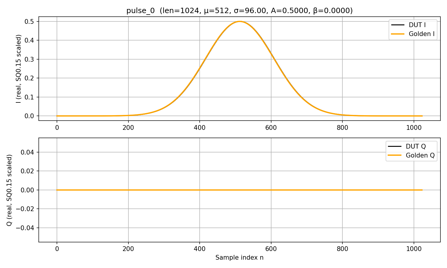
PASS: Pulse len=1024 mu=512 inv_sig2=0x00038e39 amp=16384 beta=0 use_ww=0 Am=0 wm=0 protocol+math=1, all in-phase values within 1 LSB(s) and quadrature values within 2 LSB(s) from golden.
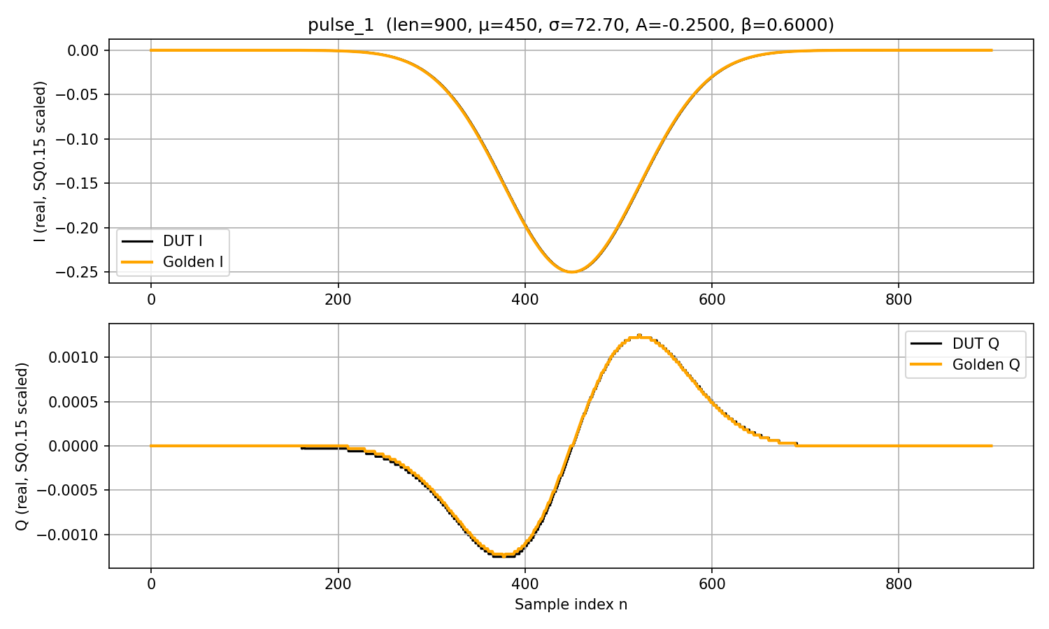
PASS: Pulse len=900 mu=450 inv_sig2=0x0006332a amp=-8192 beta=19661 use_ww=0 Am=0 wm=0 protocol+math=1, all in-phase values within 1 LSB(s) and quadrature values within 2 LSB(s) from golden.
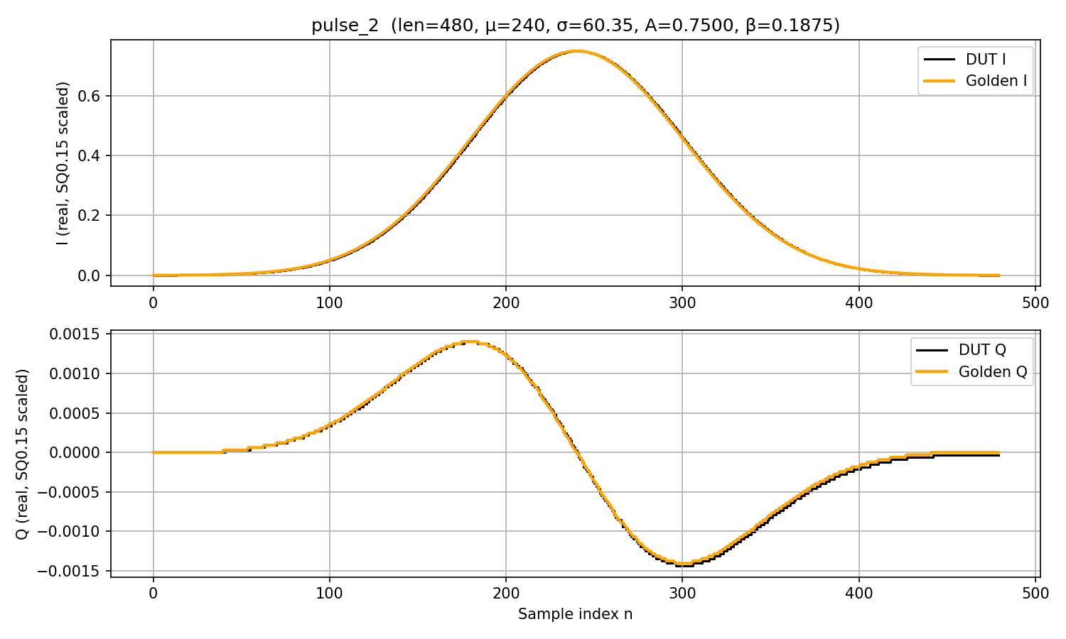
PASS: Pulse len=480 mu=240 inv_sig2=0x0008ff39 amp=24576 beta=6144 use_ww=0 Am=0 wm=0 protocol+math=1, all in-phase values within 1 LSB(s) and quadrature values within 2 LSB(s) from golden.
PASS: Pulse len=512 mu=256 inv_sig2=0x00051eb9 amp=20480 beta=8192 use_ww=1 Am=29491 wm=128 protocol+math=1, all in-phase values within 1 LSB(s) and quadrature values within 2 LSB(s) from golden.
PASS: Invalid cmd rejected. len=32 mu=32 inv_sig2=0x08000001 use_ww=0 wm=0
PASS: Invalid cmd rejected. len=2 mu=0 inv_sig2=0x20000001 use_ww=0 wm=0
PASS: Invalid cmd rejected. len=16 mu=8 inv_sig2=0x00000000 use_ww=0 wm=0
PASS: Invalid cmd rejected. len=64 mu=32 inv_sig2=0x0147ae15 use_ww=1 wm=0
PASS: All tests completed (protocol + invalid + DRAG math).
- tb_pulse_gen.sv:758: Verilog $finish
- S i m u l a t i o n   R e p o r t: Verilator 5.042 2025-11-02
- Verilator: $finish at 32us; walltime 0.043 s; speed 857.274 us/s
- Verilator: cpu 0.037 s on 1 threads; alloced 0 MB

TB validates all \(I[n]\) samples are within 1 LSB error tolerance, and all \(Q[n]\) samples are within 2 LSB error tolerance.

Plots

DRAG pulse 0:

DRAG pulse 1:

DRAG pulse 2:

Wah-Wah pulse: