Quantum Teleportation Gate

Originally published by Parity on September 19, 2026. Republished here by the author with permission.

1. Causal Locality & Cellular Automata

In this world, nothing—tangible or intangible, atoms or bits—can move faster than light, right?

We live in an era where special relativity has been verified. We believe in causality: an effect must occur after its cause. We believe that the transmission speed of any causal effect cannot exceed the speed of light in vacuum. We are familiar with Minkowski diagrams and understand that a cause must lie within the past light cone of its effect. Causal effects propagate at a finite speed and cannot ignore the distances in between. This mental model can be called “causal locality.”

The mental model of “causal locality” is so widespread that, in the field of computer science, Leslie Lamport defined the “happened-before relation” ($\rightarrow$), on which later researchers (Ahamad et al. 1995) built “causal consistency” for distributed systems: given a system with many processes, and given any two operations $A$ and $B$ satisfying $A\rightarrow B$, if every process in the system is guaranteed to observe $A$ before observing $B$, then the system is “causally consistent.” In such a system, all processes observe the same causal order.

We can study “causal locality” from a computer science perspective: cellular automata. Design a cellular automaton with the following rules:

• On a two-dimensional plane, there are two large balls, one on the left and one on the right.
• At every time step, the left ball and the right ball each toss a coin with a 50-50 probability to determine what color they will be in the next time step.
• Once a ball is “measured,” that ball freezes in its color at the moment of measurement and emits a particle toward the other ball. The particle carries the color of the frozen ball.
• A ball hit by a particle freezes into that color and absorbs the particle.

Start this cellular automaton, and measure the right ball after some time. You may observe the following result:

You will find the left ball’s color has two states:

1. State 1: after the right ball is measured, and before the particle reaches the left ball, the left ball’s color is randomly red or blue with a 50-50 probability.
2. State 2: after the particle hits the left ball, the left ball must have the same color as the right ball.

In short, after the right ball is measured, the color of the left ball is a function of the particle’s speed.

In this cellular automaton, all rules are defined over adjacent cells—each cell has eight neighbors, known as the Moore neighborhood. This limitation forces the cellular automaton to obey “causal locality,” because all changes can only be transmitted through neighboring cells. The speed of the particle is exactly “one cell per time step.” This speed is the “speed of light in vacuum” of this tiny cellular-automaton universe.

If we allow the particle to move faster, then we will be more likely to measure the left and right balls as having the same color.

Now, use our imagination to consider the case where the “time step is infinitesimally small”: the two balls randomly flash between red and blue “infinitely fast,” while the particle also moves “infinitely fast.”

Reconsidering the above experiment, we find that state 1 disappears, leaving only state 2. Using Dirac notation, let red be represented by $\ket{R}$ and blue by $\ket{B}$. When the time step is infinitesimally small, the measurement statistics of the two balls’ colors match those of the following quantum state:

\[\frac{1}{\sqrt{2}}(\ket{RR} + \ket{BB})\]

This expression says: there is a one-half probability that we will measure both balls as red, and another one-half probability that we will measure both balls as blue.

The particle moves at an “infinite speed,” causing the causal effect to violate locality and propagate at an infinite speed. This thought experiment uses a cellular automaton to demonstrate the effect of “quantum entanglement.”

Measuring one ball (cause) causes the other ball to “immediately” freeze into the same color (effect). This instantaneous propagation of causal effects regardless of distance was called “spooky action at a distance” by Einstein.

2. The Spooky Force That Worried Einstein

Local Realism

Shohei Ohtani’s splitter travels like a fastball, but drops rapidly before reaching home plate, landing in the lower-right corner of the strike zone, once again baiting the batter to swing and miss.

Is it possible to accurately calculate where a splitter will land? Common sense tells us that, by carefully considering more factors and making no computational errors, we can approach arbitrary accuracy in our result. First, consider the velocity vector of the baseball at the instant it leaves Shohei’s hand. Next, consider the angular velocity vector of the baseball at that same instant. If necessary, at every moment during the flight, consider factors such as the gravitational field, wind direction, air pressure, and humidity at its location. Consider using the most precise computer and the smallest mesh to run the most accurate finite element simulation. We believe that, by considering more factors and maintaining computational rigor, we can approach the truth.

A necessary corollary of this belief is the following: if the calculation result deviates from the truth, and we are certain that no computational error has been made, then there must be some factors that should have been considered but were missed.

Expressed in more abstract language, this belief is “realism”: everything in the universe is objectively real. If we observe a system $X$ and obtain an observation result $Y$, it is because, before the act of observation, $X$ “already” possessed a real and definite state, and our act of observation produced the result $Y$.

Imagine a simple side-scrolling game. As the player, you are located somewhere on the map. Your field of view is limited, as you can only see nearby features, such as a few walking mushrooms. However, in the background, the game system tirelessly calculates the behavior of everything on the map, regardless of whether those things appear within your field of view. This is a manifestation of “realism.”

Applied at the scale of the universe, “realism” tells us that, whether or not it is observed by a conscious subject, every location in the universe, at every moment, evolves perfectly and faithfully according to the laws of the universe.

Cunning game designers, seeking to create rich game experiences on computing platforms with limited capabilities, abandoned “realism” long ago. Super Mario Bros., released by Nintendo in 1985, does not obey “realism.” The player’s field of view is called the visible screen, while a slightly larger area is called the relevant screen. Only the game map within the relevant screen is attended to by the game system and updated frame by frame. Outside that area, monsters have not yet been born, and objects remain frozen in their “initial states.” The practice of “do not calculate what the player cannot observe” can significantly save memory and computation while having no significant effect on the gameplay experience.

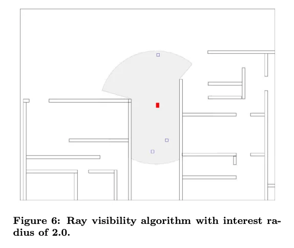
However, we fundamentally do not believe that the universe plays this trick, behaving arbitrarily in places that are not being observed. We fundamentally believe that everything in the universe evolves tirelessly with perfect precision, like perfectly interlocking gears.

Combining “realism” with “causal locality” gives us the well-known idea of “local realism”: everything that exists is objective and independent of any observation, and an event occurring in one region cannot influence another region faster than the speed of light.

If you currently hold this belief and regard it as self-evident, then you are practically one hundred years out of date. A century ago, this belief was challenged by quantum mechanics.

Challenge to Realism

In the spring of 1925, the Davisson–Germer experiment discovered that the electron-scattering phenomenon it had originally set out to investigate—which you can understand as a microscopic billiards experiment—displayed a scattering distribution far more complex than expected.

In 1926, Davisson and Germer learned of the quantum-mechanical theories of de Broglie and Schrödinger, which argued that electrons possess wave-like properties, and were encouraged by Max Born to investigate the phenomenon as wave diffraction rather than particle scattering.

In the spring of 1927, they published their experimental results: electrons scattered off the surface of a nickel crystal came back strongly only at particular angles, exactly as waves diffracted by the crystal lattice would.

The fact that particles possess wave-like properties is itself a challenge to realism. A particle, at any given moment, can only actually exist in one place, right? Semantically, a particle is a localized existence. Quantum mechanics, however, says that a particle’s position does not possess one single, definite existence. Instead, it is probabilistically spread across space and described by wave theory.

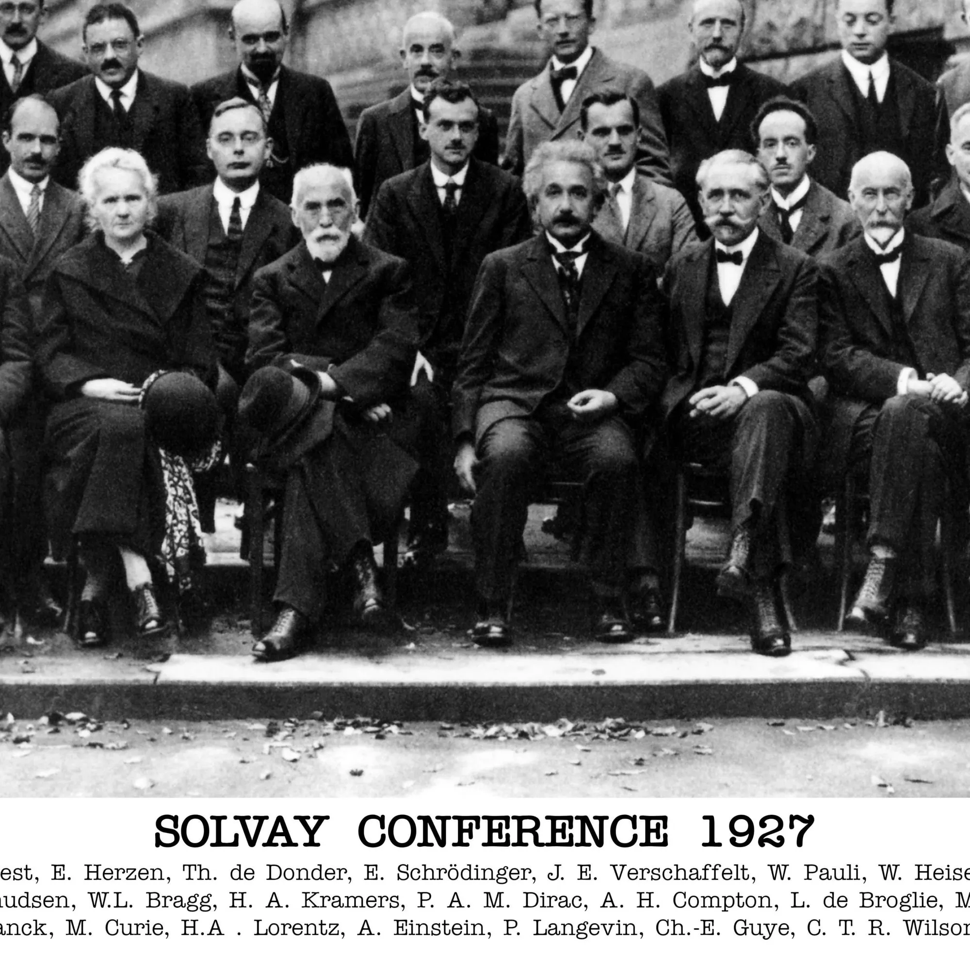
In October 1927, at the star-studded Fifth Solvay Conference in Brussels, with the theme “Electrons and Photons,” Einstein and Bohr debated whether quantum mechanics could completely describe all behavior in the universe. Einstein believed it could not; Bohr believed it could. In response to the electron-diffraction experiment, Einstein proposed a thought experiment:

• Prepare a system consisting of an electron gun, a slit, and an imaging screen.
• Quantum mechanics claims that the universe can tell us only “the probability that, after passing through the slit, the electron will appear at a particular location on the screen.” Einstein believed that this inability to provide an exact position, and its ability to provide only probabilities, resulted from some factors that should have been considered but were missed. Recall our earlier discussion of where Shohei Ohtani’s splitter would land.
• If we carefully observe tiny changes in the slit while the electron is passing through—for example, the slight recoil of the slit when the electron strikes it—we can obtain more information beyond the limits of quantum mechanics, which would help us infer the electron’s trajectory. Recall our earlier discussion about wind direction, air pressure, and humidity.

Bohr replied that if we precisely observe the recoil of the slit—its momentum—then the uncertainty principle of quantum mechanics tells us that we can no longer possess precise information about the slit’s position. Since the diffraction pattern depends on the position of the slit, if the slit’s position becomes uncertain, the diffraction image becomes disordered. The pattern would disappear.

Einstein was not satisfied. He believed that there must be some missing factors. The idea that there could only be “probability” and no certainty had to be a defect in human physics. The universe should not evolve in an uncertain way.

Heisenberg recalled:

• Einstein: “God does not play dice.”
• Bohr: “It cannot be for us to tell God how he is to run the world.”

Challenge to Locality

At the same conference, Einstein proposed another thought experiment:

• Prepare a system consisting of an electron gun, a small aperture, and an imaging screen.
• Quantum mechanics says that after an electron passes through the aperture, it forms a hemispherical “electron wave,” and the electron’s possible location can be described by the shape of this wave. Although the electron wave spreads in every direction, experiments tell us that if the electron gun emits one electron, only one point will appear on the imaging screen.
• If the electron wave is the electron’s physical reality after it passes through the aperture, this reality, taking the shape of a wave and spreading throughout space, eventually becomes a single point upon reaching the screen. This “collapse” from a wave to a point would require some instantaneous method of transmitting information that disregards distance: the point at which the electron is detected must instantly notify every other location on the screen, “Hey, the electron is here! You are not allowed to detect it there!”
• Such a distance-defying force violates locality. It is a “spooky action.”

Quantum mechanics challenges both “realism” and “locality”: things possess no definite reality and can only be described in terms of probability, while a nonlocal action at a distance governs how those probabilities change.

Many years after the conference, Einstein remained dissatisfied. The 1935 EPR paper was an attempt to challenge quantum mechanics. Imagine two particles, $A$ and $B$, that interact and then separate: their total momentum is zero, and the distance between them is also definite. We may freely choose whether to measure the momentum or the position of $A$. If we choose to measure the momentum of $A$, by applying conservation of momentum, we can instantly determine the momentum of $B$. If we choose to measure the position of $A$, because the distance between the two is definite, we can instantly determine the position of $B$ without measuring it.

Based on this result, if we believe in “locality”—that measuring $A$ cannot instantaneously affect $B$—the momentum and position of $B$ must each be real and definite. Only then could their values be known instantly without being measured. Finally, because quantum mechanics claims that only one of position and momentum can be described precisely at a time, quantum mechanics must be incomplete: there must be some hidden factors that should have been considered.

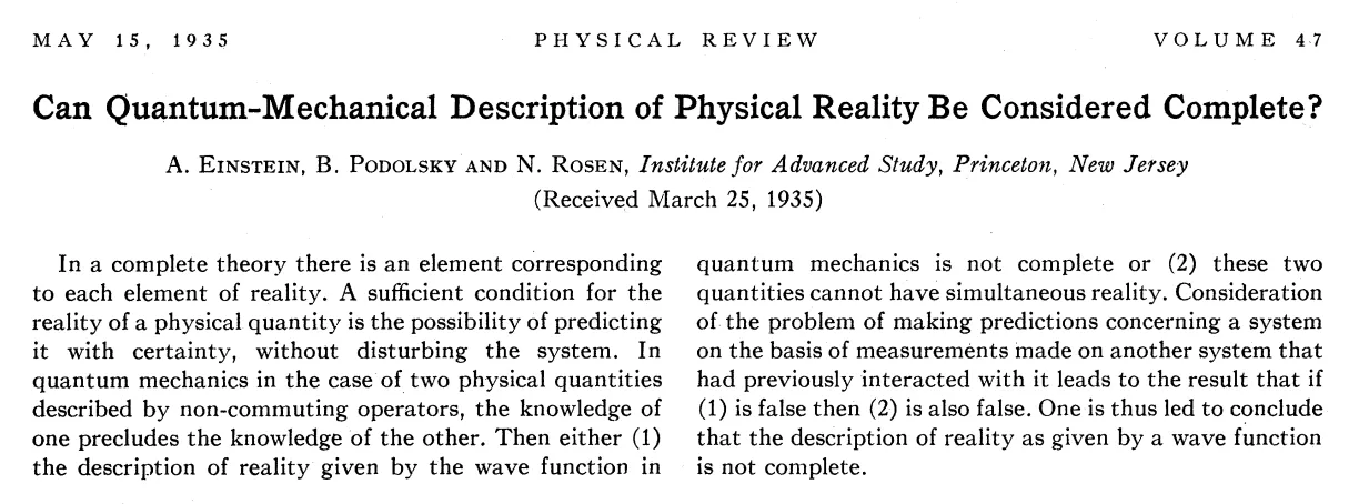
Call these hidden factors “hidden variables,” and the resulting theory is called a “local hidden-variable theory” (LHVT).

In 1951, the EPR paper’s thought experiment was reformulated by David Bohm. After two particles that had been bound together separated, conservation of angular momentum meant that measuring the spin value of one particle along a certain axis would reveal the spin value of the other particle along the same axis. Spin values are discrete, $\pm 1$, and are easier to measure precisely in experiments than the continuous position and momentum.

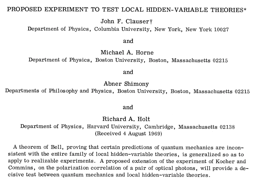
In 1964, John Bell turned this thought experiment into a falsifiable inequality, allowing LHVT to be falsified using statistical values from experimental data. In 1969, John Clauser and others removed one strict condition required by Bell’s thought experiment—that measurements along the same direction on the two sides be perfectly anticorrelated, which no real source, analyzer, or detector achieves—and designed a version that was easier to test experimentally, together with a new inequality known as the CHSH inequality.

To date, Bell inequalities (CHSH and its variants) have been violated in several dozen experiments, e.g., Freedman & Clauser 1972, Aspect et al. 1982, Weihs et al. 1998, Hensen et al. 2015.

These experimental results suggest that we abandon our belief in “local realism.” In its place, there exists in the universe an action-at-a-distance force that can transmit causal effects instantaneously. It is precisely this action-at-a-distance force that is responsible for state updates in quantum-entangled systems.

Recall the cellular automaton from earlier. With the particle moving at infinite speed, we could squint and view the two balls as a quantum-entangled system. When the color of one ball is measured, the color of the other ball is frozen into the same color at that very instant.

3. Harnessing the Spooky Action

The CHSH Test and Inequality

Let’s study the CHSH inequality:

\[\langle a_1 \cdot b_1 \rangle+\langle a_1 \cdot b_2 \rangle+\langle a_2 \cdot b_1 \rangle- \langle a_2 \cdot b_2 \rangle \leq 2\]

Picture Alice and Bob as two experimenters separated in space. Between them is a pair of twin particles bound together. Suddenly, the pair splits apart, and each particle flies toward one of the experimenters. The experimenters are interested in the spin values of these particles, and each chooses 2 directions along which to perform measurements. For example, Alice’s first direction may be the vertical direction perpendicular to the ground, while her second direction may be parallel to the ground to her right-hand side. The two experimenters may freely choose whichever directions they prefer.

Any measured spin value of a particle can only be +1 or -1:

• +1 means “the particle was measured to spin along the measurement direction!”
• -1 means “the particle was measured to spin in the direction opposite to the measurement direction!”

Now let’s formalize our discussion with variables. Alice’s two measurement directions are $A_1$ and $A_2$. The spin value obtained by measuring along $A_1$ is $a_1$, while the spin value obtained by measuring along $A_2$ is $a_2$. Thus,

\[a_1,a_2\in\{+1,-1\}\]

Bob’s directions are $B_1$ and $B_2$, and his results are

\[b_1,b_2\in\{+1,-1\}\]

Alice and Bob perform this experiment many times, independently record their measurement results, and finally run a statistical analysis.

In each experimental run, there are only 4 possible combinations of Alice’s and Bob’s measurement directions:

\[A_1B_1,\quad A_1B_2,\quad A_2B_1,\quad A_2B_2\]

In each run, the product of Alice’s and Bob’s measurement results takes one of two possible values: $+1, -1$.

The left-hand side of the CHSH inequality is this expression:

\[\langle a_1 \cdot b_1 \rangle+\langle a_1 \cdot b_2 \rangle+\langle a_2 \cdot b_1 \rangle- \langle a_2 \cdot b_2 \rangle\]

where $\langle\ \rangle$ denotes the statistical average. What do these averages mean? Take $\langle a_1\cdot b_1\rangle$. Across all experimental runs, select those where Alice and Bob used the measurement combination $A_1 B_1$. Calculate the product of their results from each selected run, then take the average.

Therefore, the above expression amounts to calculating four average values from experimental data, adding the first three together, and subtracting the fourth.

If we believe in “local realism,” after the particles separate, they no longer exchange information. Each particle carries its own “real values” toward its respective experimenter. Imagine that when the particle flying toward Bob separates from its twin, it has already “decided”: if Bob measures along direction $B_1$, I will give him the result +1; if he measures along $B_2$, I will give him the result -1.

By enumerating all possible “decisions” that the pair of twin particles could make, the authors of the CHSH paper found that “local realism” leads to:

\[\langle a_1 \cdot b_1 \rangle+\langle a_1 \cdot b_2 \rangle+\langle a_2 \cdot b_1 \rangle- \langle a_2 \cdot b_2 \rangle \leq 2\]

However, to date, several dozen experiments have produced data that violate this inequality.

The CHSH Game

Some researchers are not so much interested in “local realism.” After all, they—or their academic advisors—were already persuaded by Bohr back in the days of the Solvay conferences. Their focus is on quantum information technology: What use does this spooky action have in information technology?

In the early 2000s, the experimental test of the CHSH inequality was reformulated as a cooperative information game:

• Alice and Bob are separated and cannot communicate.
• A neutral referee gives each of them a random bit, with values $x$ and $y$, and asks each of them to return one bit to the referee, with values $a$ and $b$.
• Alice and Bob win together:
  • If $(x, y) = (1, 1)$, $a$ and $b$ must differ.
  • If $x$ and $y$ take any of the other 3 combinations, $a$ and $b$ must be the same.

Compress the conditions above into a single equation:

\[a \oplus b = x \land y\]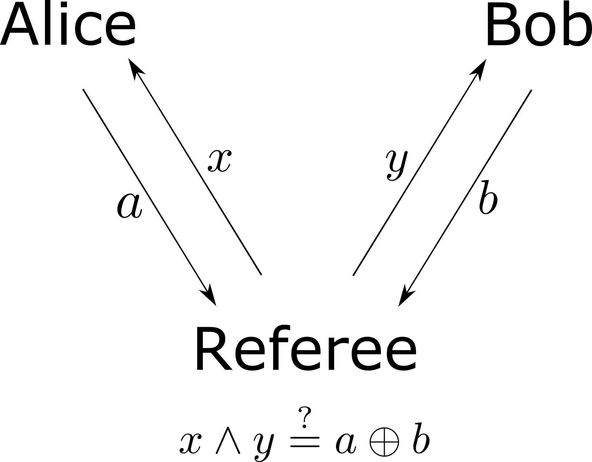

Interestingly, because quantum entanglement does not count as communication, the game allows Alice and Bob to share and operate on a pair of entangled particles. Imagine the two balls from our earlier cellular automaton: Alice and Bob may each hold one of them.

How should Alice and Bob play? Consider the challenge. When $(x, y) = (1, 1)$, the two must give different answers; in the other three cases, they must give the same answer. However, they have no way to communicate and determine which case they are in. Therefore, without leveraging quantum entanglement, their best strategy is very simple: before the game begins, they agree that no matter what happens, they will both return the same answer. Their winning probability is 75%. It is impossible to get any higher than that.

What if they leverage quantum entanglement? Alice and Bob can prepare a pair of entangled particles in the following state:

\[\frac{1}{\sqrt{2}}( \ket{00} + \ket{11} )\]

For this pair of particles, as long as both sides measure along the same direction (all the directions in this example lie in one plane), no matter who measures first or what result is obtained, the measurement outcomes on the two sides will always agree.

Alice and Bob then agree on the following strategy:

• Each chooses two measurement directions. Alice’s directions are $A_1,A_2$, while Bob’s directions are $B_1,B_2$.
• During the game:
  • If Alice receives the random bit $x=0$, she measures her entangled particle along direction $A_1$, obtaining the result $a_1$. If she receives $x=1$, she measures along direction $A_2$, obtaining the result $a_2$.
  • If Bob receives $y=0$, he measures along direction $B_1$, obtaining the result $b_1$. If he receives $y=1$, he measures along direction $B_2$, obtaining the result $b_2$.
• As in the CHSH test, any measurement result can only be +1 or -1.
• Alice and Bob each submit their measurement result to the referee as their answer.

To maximize the winning probability, what directions should $A_1,A_2,B_1,B_2$ be?

The rules of the game tell us that when $x=y=1$, Alice and Bob must give different answers to win. In other words, the product $a_2 \cdot b_2$ must be negative. Therefore, Alice and Bob are effectively trying to maximize the following statistical quantity:

\[\langle a_1 \cdot b_1 \rangle + \langle a_1 \cdot b_2 \rangle + \langle a_2 \cdot b_1 \rangle - \langle a_2 \cdot b_2 \rangle\]

This is exactly the left-hand side of the CHSH inequality!

Skipping the derivation—which involves wave-function basis projection, beyond the scope of this article—we find that Alice and Bob can choose the following measurement directions to maximize their winning probability:

• A1 = 0°
• A2 = 90°
• B1 = 45°
• B2 = -45°

These choices lead to a winning probability of $\cos^2(22.5^\circ)\approx 0.8536$, or 85.36%, which is greater than the maximum winning probability of 75% when quantum entanglement is not used.

Note that Alice and Bob each measure the entangled particle in their possession. The act of measurement “consumes” the particles: after they are measured, they are no longer entangled.

This notion of consumption suggests that entangled particles can be considered as an engineering resource to perform nonlocal operations on quantum states.

Quantum Teleportation Circuit

A more generalized goal than winning the CHSH game is: how to transfer a piece of quantum information from Alice in one location to Bob in another location using entangled particles?

To clarify, even with quantum entanglement, we cannot achieve faster-than-light transmission of classical information. However, by consuming a pair of entangled particles, we can transfer the quantum state held by Alice to Bob. Notice that after the transfer, Alice no longer possesses the quantum state, as we are confined by the no-cloning theorem.

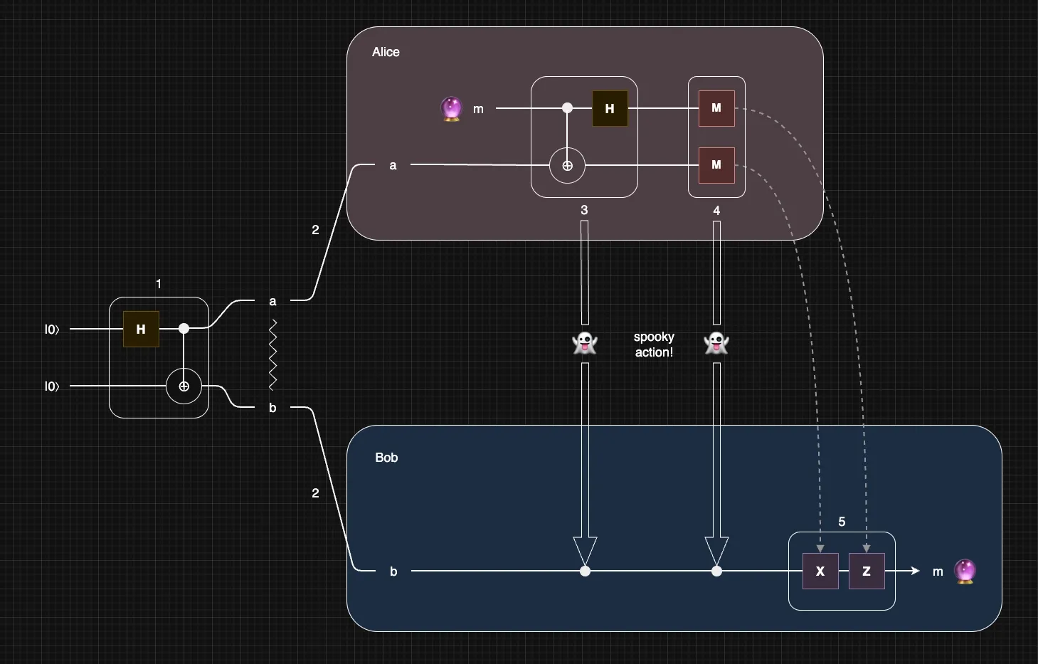
At a basic level, the transfer involves 5 steps:

1. Prepare a pair of entangled particles, $a$ and $b$, in the so-called Bell state. The measurement results on these two particles are either both 0 or both 1, with equal probability.

\[\frac{1}{\sqrt{2}}(\ket{00}+\ket{11})\]

1. Distribute $a$ to Alice, and $b$ to Bob, while keeping $a$ and $b$ entangled.
2. Alice entangles her particle with the message quantum state $m$. At this point, the three quantum states $a$, $b$, and $m$ are all entangled together.
3. Alice measures $a$ and $m$, thereby consuming $a$ as a resource, and collapsing $m$.
4. Alice communicates the measurement results—classical information—to Bob through a classical communication channel. Based on the information received, Bob performs the corresponding quantum gate operations on $b$ as a correction. Now, Bob possesses the message quantum state $m$.

The entire process can be represented by the following quantum circuit. Quantum gate symbols such as the $H$ gate and the $X$ and $Z$ gates are beyond the scope of this article; the $\oplus$ symbol representing the CNOT gate will be explained below.

Scaling Challenges of Quantum Computing

In scaling quantum computers, one of the most basic metrics is the physical qubit count: the number of physical qubits that a computing platform can prepare, maintain, and operate at the physical level.

Over the past thirty years, the number of qubits on a single (monolithic) platform has continued to increase. In recent years, neutral-atom platforms in particular have scaled at the fastest rate, as shown in the figure below.

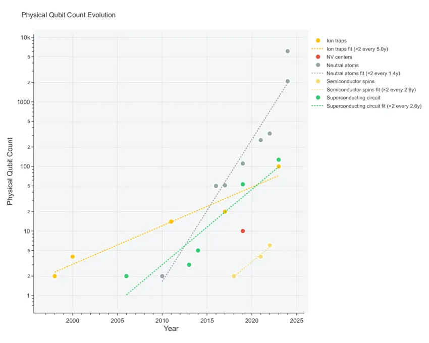
However, if we require that the physical qubits be flexibly allocatable to perform 1-qubit gates and 2-qubit gates, the limit today is in the hundreds of physical qubits on a single platform. For example:

• 256 qubits in Logical computation demonstrated with a neutral atom quantum processor.
• 280 qubits in Logical quantum processor based on reconfigurable atom arrays.

Across different qubit types, single-platform scaling encounters various difficulties.

Superconducting-Circuit Platforms

Superconducting-circuit platforms operate superconducting circuits at low temperatures as qubits, and use the two lowest energy levels of the circuit as $\ket{0}$ and $\ket{1}$. The energy gap is commonly around 20 µeV, corresponding to an excitation frequency of approximately 5 GHz. Therefore, transitions between the two energy levels rely on 5 GHz microwave signals.

However, a 5 GHz signal corresponds to a wavelength of approximately 3 centimeters in a waveguide, which is on par with the scale of the entire circuit system, leading to significant crosstalk: a signal originally intended to drive a specific qubit spills over and affects other qubits. In practice, excitation frequencies of neighboring qubits are staggered through deliberate control of circuit dimensions. However, one limitation of this design is that if qubits A and B are adjacent, and A’s excitation frequency is lower than B’s, then A’s $\ket{0} \leftrightarrow \ket{1}$ frequency may be close to B’s $\ket{1}\leftrightarrow\ket{2}$ frequency. As a result, when the signal driving A spills over to B, it may push B into $\ket{2}$, causing information loss. This limits the number of excitation frequencies that can be accommodated within finite bandwidth.

Moreover, the entire superconducting circuit system typically operates at approximately 0.015 K and must be placed inside a specially designed refrigerator. More qubits require more control signal lines and readout signal lines to be routed into the refrigerator, bringing in more heat and increasing noise. Noise destroys quantum states.

Trapped-Ion Platforms

Trapped-ion platforms cool ions to low temperatures using methods such as Doppler cooling and sideband cooling, and confine them in potential wells formed by alternating electric fields (Paul traps, e.g., Cirac & Zoller 1995 and Monroe et al. 1995) or by a static electric field combined with a strong magnetic field (Penning traps, e.g., Jain et al. 2018). Each ion constitutes an individual qubit. In addition to their individual quantum states, these qubits form collective vibrational modes within the shared electromagnetic field. By coupling their quantum states to these collective vibrational modes, the qubits can become entangled for the purpose of performing 2-qubit gate operations.

However, once the number of qubits increases, the collective vibrational modes become more complex, and the modes crowd together, making unintended entanglement more likely and causing errors in computation. Therefore, researchers moved on from building one large trap shared by all qubits to building multiple independent smaller traps. This approach requires the ability to transport ions between traps, increasing architectural complexity. The transport process also generates noise that interferes with the quantum states.

Neutral-Atom Platforms

Neutral-atom platforms cool neutral atoms to low temperatures using methods such as magneto-optical trapping and sideband cooling. Each atom is confined by an optical tweezer at a specific position, forming a matrix of qubits.

Increasing the number of qubits requires scaling up the optical systems that control them: these systems must simultaneously operate large numbers of optical tweezers and laser beams for excitation and readout, while maintaining high precision in frequency, phase, and spatial positioning.

After cooling is completed, the neutral atoms must be rearranged into a matrix with optical tweezers. The more qubits there are, the longer the rearrangement takes and the farther the atoms must be transported, increasing noise.

To create quantum entanglement, neutral atoms are excited into highly excited Rydberg states. Through van der Waals forces, an atom in a Rydberg state suppresses the probability of nearby atoms getting excited to the same state, a mechanism known as the Rydberg blockade, which causes neighboring atoms to become entangled. However, as the number and density of qubits increase, van der Waals forces are more likely to affect nearby atoms that should not be affected, causing gate errors.

If we scale up the number of qubits without increasing density, the overall array becomes larger, increasing the distance and time required for rearrangement and atom transport, thereby increasing noise.

Quantum Supercomputer

Consider the evolution of classical computers. Because complex scientific simulation problems exceeded the capabilities of any single machine, massively parallel processing emerged in the 1980s and 1990s. Supercomputers such as those built by Cray at the time connected as many as two thousand processors together.

Quantum computing today remains at a very early stage: no single quantum machine has yet provided commercial application value that classical computers cannot provide. To accelerate scaling, researchers began to ask: as with classical supercomputers, how can we connect multiple small quantum platforms to build a quantum supercomputer?

This mission involves challenges that do not exist in classical supercomputers: quantum states cannot be copied, and physical transportation exposes them to noise and decoherence. Ideally, multiple quantum platforms would share quantum states and operate on those states while avoiding the physical movement of qubits as much as possible. This would allow multiple quantum platforms to be “virtualized” into a single ultra-large platform with effectively a great number of qubits to unlock new computational problems beyond the capabilities of any classical computer.

Nonlocal Gates

One of the keys lies in harnessing the spooky action to build nonlocal gates.

Consider a classical computer. A logic gate occupies a specific location and area on a chip. Through the materials used in the gate, its structural design, and other factors, the gate maintains the intended logical relationship between its input and output signals. For example, if we want to perform an XOR operation $\oplus$ on two classical bits, we must transmit the signals carrying those two bits to the input ports of a single XOR circuit, positioned at a particular locality in the circuit system, and capture the result at its output port.

A nonlocal gate, in contrast, can perform a logical operation on multiple input data located in different places, despite the distance between them. Imagine in Laboratory 101 a quantum platform contains a qubit $a$ in quantum state $x$, while in the neighboring Laboratory 102 a quantum platform contains a qubit $b$ in quantum state $y$. Through a nonlocal gate, without moving either $a$ or $b$, we can “snap our fingers” from afar and make the quantum state of $b$ become $x\oplus y$, at the cost of one pre-shared entangled pair and one classical bit sent in each direction.

Let’s study the Remote CNOT described in Eisert et al. 2000.

CNOT, or controlled-NOT, is a 2-qubit gate. It has two inputs, control in and target in, and two outputs, control out and target out. Its rule is simple: when control in is $\ket{1}$, target in is flipped (more precisely, an $X$ gate is applied) to produce target out; otherwise, target out is equal to target in. CNOT is one of the most basic logic gates and is included in the universal gate sets of many computing platforms.

A regular CNOT operates on two qubits that are adjacent in physical space—that is, local. A Remote CNOT goes beyond locality:

• Alice and Bob are separated and each hold one qubit, $a$ and $b$.
• In addition, Alice and Bob each hold one qubit of an entangled qubit pair, $e_a$ and $e_b$.
• Through the Remote CNOT, Alice and Bob can perform CNOT($a$, $b$), using $a$ as the control and $b$ as the target. If $a$ is $\ket{0}$, $b$ remains unchanged; if $a$ is $\ket{1}$, $b$ is flipped.

Consider the circuit:

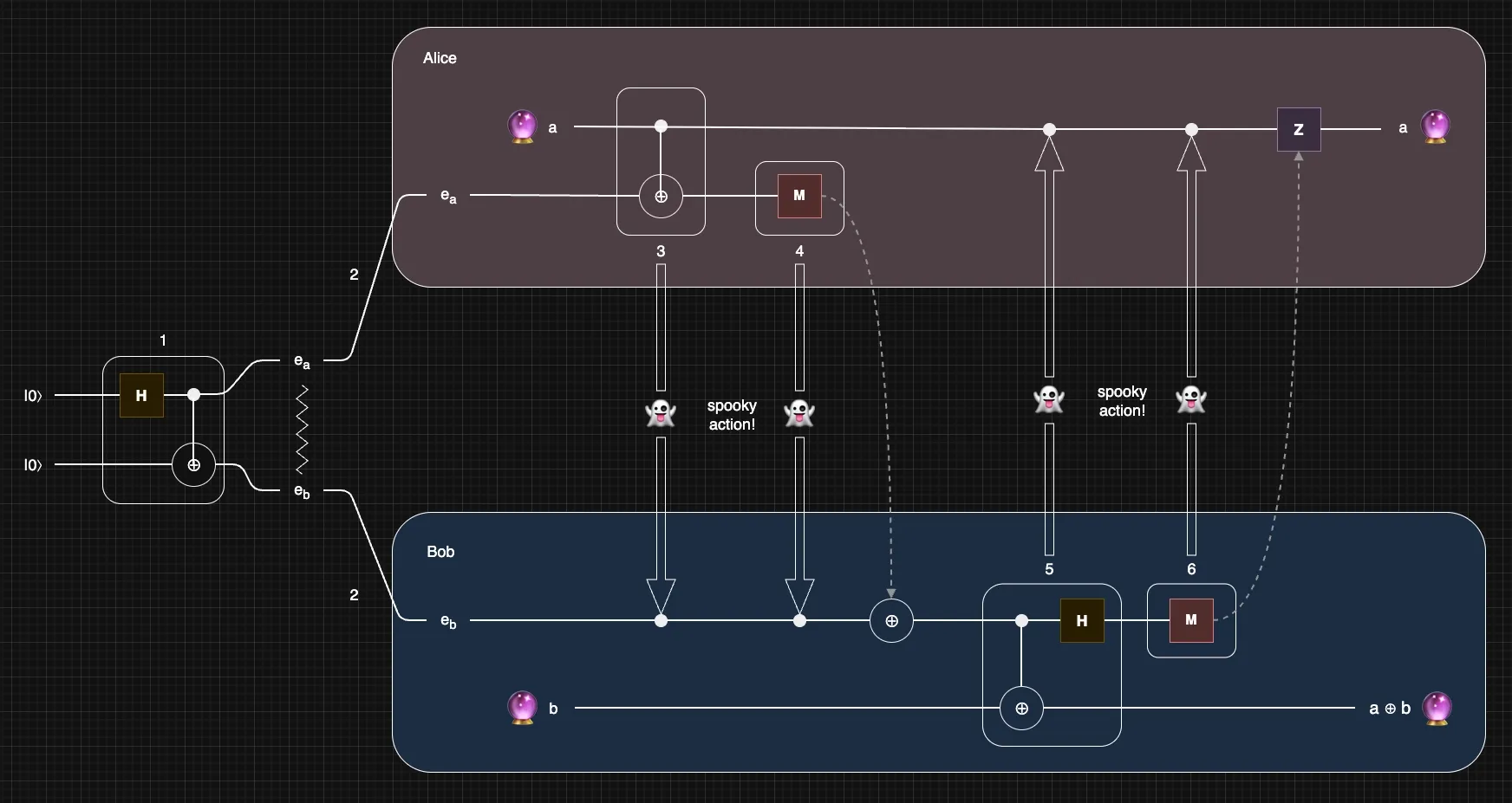
The entire procedure consists of 6 steps:

1. Prepare an entangled pair in the Bell state, with the two qubits denoted as $e_a$ and $e_b$.

\[\frac{1}{\sqrt{2}}(\ket{00}+\ket{11})\]

1. “Distribute” $e_a$ and $e_b$ to Alice and Bob, respectively. How to “distribute” without physically transporting the qubits will be discussed below.
2. Alice entangles her qubit $a$ with $e_a$.
3. Alice measures $e_a$, thereby consuming it, and communicates the measurement result to Bob through a classical channel. Bob then uses that information as the control bit to run a CNOT on $e_b$, a local correction.
4. Bob entangles his qubit $b$ with $e_b$.
5. Bob measures $e_b$, thereby consuming it, and communicates the measurement result to Alice through a classical channel. Alice then uses that information as the control bit to run a CZ (controlled-Z) operation on $a$, a local correction.

After these steps, the qubits held by Alice and Bob have undergone a joint state transformation equivalent to that of a local CNOT:

\[\ket{a}\ket{b}\longmapsto \ket{a}\ket{a\oplus b}\]

The resources consumed by this procedure are:

• 1 ebit of shared entanglement
• 1 cbit of classical communication in each direction

Overall, pre-shared entanglement is a consumable resource. By consuming entanglement, exchanging classical measurement results, and applying local correction operations, we can have two spatially separated qubits jointly execute a logic gate without physically transporting either qubit.

4. Commercial Ambition

Entanglement Swapping

For both the quantum teleportation circuit and the nonlocal gate, steps 1 and 2 are “prepare an entangled qubit pair; distribute the entangled qubits to the two parties.” The question is: how do we distribute the entangled qubits without physically transporting them?

In fact, we do not distribute the qubits. It is not the case that $e_a$ and $e_b$ are prepared somewhere and then distributed to Alice and Bob.

The practical approach is to use photons as “flying qubits” to transform a pair of qubits already held by Alice and Bob into an entangled state.

More specifically, neutral-atom and trapped-ion platforms prepare entanglement resources in the following way:

1. Alice and Bob each allocate one qubit, denoted as $e_a$ and $e_b$, to be transformed into an entanglement resource.
2. Repeat the following steps until success:
   1. Alice and Bob each excite the qubit in their possession, causing it to emit a photon, denoted as $p_a$ and $p_b$. The qubit–photon pair $e_a - p_a$ is entangled, and the pair $e_b - p_b$ is also entangled. The specific method of excitation will be discussed below.
   2. For either party, after successful entanglement, the state of the qubit–photon pair can be described by the following expression: $\frac{1}{\sqrt{2}} \left( \ket{0}_e\ket{H}_p + \ket{1}_e\ket{V}_p \right)$. This means that there is a 1/2 probability of measuring “qubit in 0, photon in horizontal polarization,” and a 1/2 probability of measuring “qubit in 1, photon in vertical polarization.”
   3. Send the two photons $p_a$ and $p_b$ to an interference station. Here, we perform interference with the two photons so that the spatially separated qubits $e_a$ and $e_b$ become entangled. This involves 2 steps:
      1. Send the 2 photons into a beam splitter with 2 inputs and 2 outputs. Our goal is to “mix” them so that the 2 output photons cannot be individually traced back to their corresponding input photons. Functionally, this is analogous to a cryptocurrency mixer. If successful, the 2 photons can be treated as a joint system.
      2. Measure the polarization directions of the 2 photons. This measurement procedure is called a Bell-state measurement (BSM). When the measurement result shows one of the specific combinations of polarization directions, we can declare, or herald, that $e_a$ and $e_b$ have successfully entered an entangled state. If we fail to see the specific combinations in our BSM result, we return to step 2a and repeat until this step succeeds.

This procedure transforms two qubit–photon entanglement pairs, $e_a - p_a$ and $e_b - p_b$, into one qubit–qubit entanglement pair $e_a - e_b$. Proposed in 1993, this procedure is called entanglement swapping.

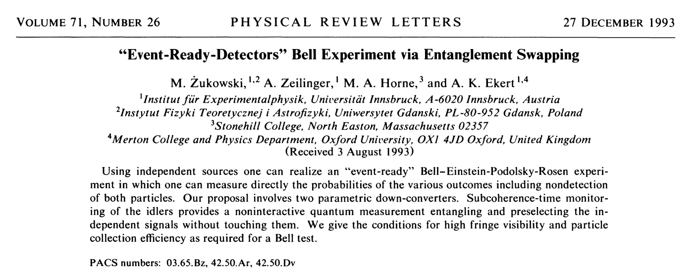
We are still missing a piece of the puzzle: in step 2a, how is the qubit–photon entanglement generated?

Qubit–Photon Interface

How can a qubit $Q$ be “excited” so that the photon $P$ it emits becomes entangled with $Q$?

Consider a neutral-atom or trapped-ion qubit $Q$ in free space. A laser pulse excites $Q$, which then decays and emits a photon $P$. If the excited $Q$ has multiple decay paths available, the energy level of $Q$ after emission and the state of $P$, such as its polarization direction, may become entangled.

However, carrying out this process in free space involves at least the following 3 variables:

1. To which energy level will the excited $Q$ decay, and what frequency will $P$ have?
2. In which direction will the excited $Q$ emit $P$?
3. How much time will pass between excitation and emission?

For Variable 1, we want $Q$ to return to either $\ket{0}$ or $\ket{1}$ after emission. Any quantum platform, using neutral atoms or ions of a particular element under a particular external magnetic field, defines its particular ${ \ket{0}, \ket{1} }$ as its computational subspace. For classical computing, the “computational subspace” is the pair of voltage levels {0 V, 1.2 V} on a CMOS chip, interpreted as logical 0 and logical 1, respectively. If $Q$ ends up outside ${ \ket{0}, \ket{1} }$ after emission, this constitutes a leakage from the computational subspace. If the leakage cannot be corrected, we lose quantum information.

For Variable 2, radiation in free space may be carried out randomly in many different directions. When the direction is uncontrollable, we have low efficiency in photon collection.

For Variable 3, the emission time in free space is also random. More specifically, the waiting time until decay follows an exponential distribution. A cavity, by contrast, can shorten and shape the photon’s wave packet, making it easier for the photons from Alice and Bob to overlap at the beam splitter and allowing a higher repetition rate.

To make the decay path, emission direction, and timing more controllable, researchers use cavities to alter the electromagnetic environment surrounding the qubits. This is an application of the Purcell effect. In 1946, Edward Purcell, while studying nuclear magnetic resonance, proposed in a brief conference abstract that if an emitter is placed inside a cavity and the cavity’s mode resonates with the emission transition, the rate of emission is enhanced. This cavity-induced modification of the spontaneous-emission rate is known as the Purcell effect.

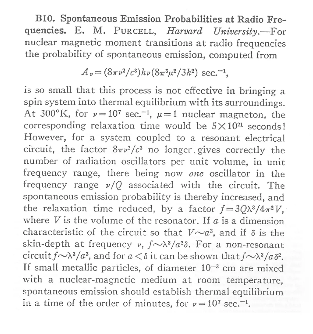
By constructing the cavity from two opposing mirrors and carefully designing the cavity geometry and qubit placement, we can better control the decay path, direction, and timing of $Q$’s emission. If one mirror is made slightly more transmissive, it can serve as the “egress,” allowing $P$ to leave the cavity, enter an optical fiber, and travel to the interference station. Wilk et al. 2007 is one of the early representative works that realized such a design.

The Ambition of Nu Quantum: Datacenter-Scale Distributed Quantum Computing

Nu Quantum is a British company spun out of the Cambridge Cavendish Laboratory in 2018. It aims to become the “Cisco” of quantum datacenters in the future by providing networking solutions that connect quantum computers and realize distributed fault-tolerant quantum computing.

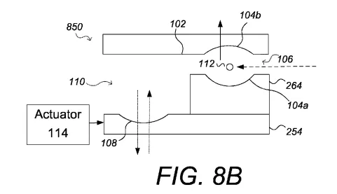
Nu Quantum uses cavities as qubit–photon interfaces (QPIs). The figure below comes from Nu Quantum’s PCT patent application WO2023073379A1; a UK patent in the same family, GB2612578B, was granted in 2024.

A walkthrough of the main components in the design:

• 104a and 104b are the two mirrors that form the cavity.
• 112 is the qubit.
• 106 is the cavity itself, the gap between 104a and 104b; the laser pulse that excites the qubit enters from the side, along the dashed arrow on the right.
• 114 on the left is a mechanical actuator. Using Pound–Drever–Hall frequency stabilization, together with mirrors 102 and 108 (rigid extensions of the cavity mirrors 104a and 104b), the distance between the mirrors is dynamically locked, which maintains the stability of the cavity-mode frequency.

According to a paper published by the team in 2025, the cavity is approximately 370 µm long, with a waist of approximately 5 µm. A 2024 press release further stated that the cavity length could be locked to within 0.08 nm. For the 780 nm transition commonly used with rubidium-87 neutral-atom qubits, this corresponds to a frequency error of approximately $2\times10^{-5}$% (about 80 MHz).

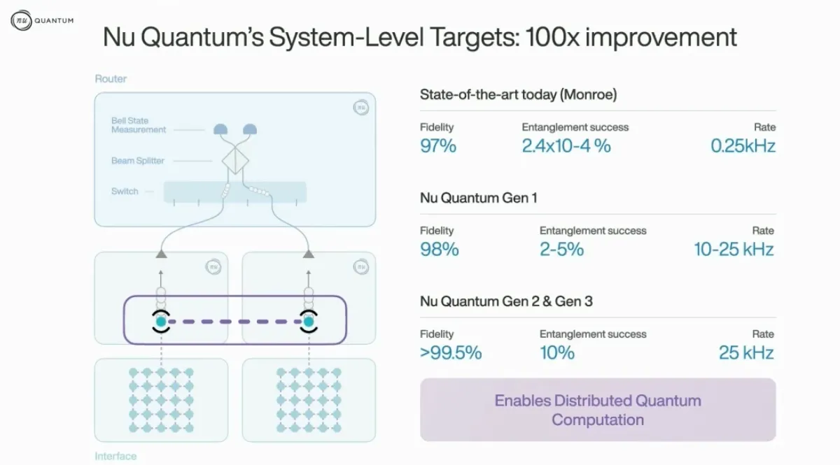
O’Reilly et al. 2024, from Monroe’s group, represents the state of the art, achieving a successful entanglement generation rate of 250 events per second, or 250 Hz. Because quantum supercomputers will require large amounts of entanglement resources, under continuous replenishment, to perform nonlocal gates, the entanglement generation rate is critical. One of Nu Quantum’s near-term goals is to increase this rate by another 2 orders of magnitude.

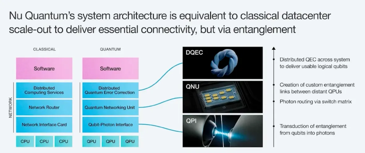
Nu Quantum’s broader goal is to virtualize multiple quantum platforms—also known as quantum processing units, or QPUs—under the roof of a single datacenter as one distributed platform. At present, their networking solution supports only trapped-ion and neutral-atom platforms. The solution involves 3 layers:

1. The QPI forms the lowest layer. Installed within each quantum platform, it generates the qubit–photon entanglement described above and outputs photons.
2. The next layer is the Quantum Networking Unit, or QNU. It routes and pairs photons arriving from different QPIs, repeatedly performs Bell-state measurements until successful heralding, and creates shared nonlocal entanglement resources between arbitrary pairs of QPUs.
3. The upper layer is Distributed Quantum Error Correction, or DQEC (refer to their 2025 paper). It performs error detection and correction across multiple QPUs, allowing the physical qubits distributed among them to be abstracted into functional logical qubits to be used by quantum software.

The Ambition of CavilinQ: High-Rate Quantum Interconnects

CavilinQ, founded in 2025, shares the long-term vision of joining many separate quantum computers into one far larger machine through photonic links. CavilinQ is focusing on raising the bar on the rate and fidelity of QPIs so that photons from separate processors can be interfered and the distant qubits entangled with a higher interconnecting bandwidth.

The crux of the QPI is the interface between a qubit and the photon it emits. CavilinQ builds cavity-based interfaces that make this emission fast, directional, and well-timed, making the subsequent heralding step faster and more reliable. The team has integrated more than 5 different types of cavities with quantum memories, a hands-on experience that is rare in the field and central to making interconnects work in practice.

Recall that in a QPI, the cavity’s resonant-mode frequency must be brought as close as possible to the decay transition of the qubit. The closer the two frequencies are, the greater the probability of inducing the qubit to undergo the desired decay. One key metric is the cavity finesse, a dimensionless ratio. Raising the finesse (lowering the losses inside the cavity) and shrinking the beam waist strengthen the coupling between the qubit and the cavity mode, so that more photons go into the cavity mode and then out through the egress mirror.

A recent paper by its team presents a new cavity fabrication process that achieves a finesse of about 0.9 million at a wavelength of 780 nm. A brief description of that fabrication process is as follows:

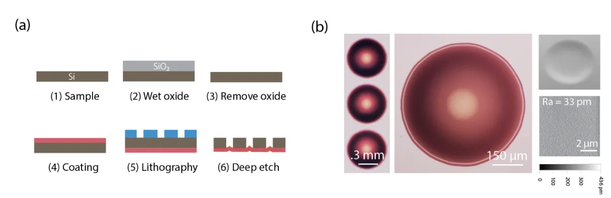
1. Smooth the surface of a silicon wafer.
2. Use ion-beam sputtering to deposit a coating on one side of the silicon wafer. The coating consists of dozens of alternating layers of high- and low-refractive-index materials, creating high reflectivity within the target frequency range.
3. Flip the silicon wafer over, apply photoresist, and perform silicon etching. The silicon substrate beneath the openings in the photoresist pattern is etched through, exposing the back side of the coating. As a result, the coating becomes suspended, and its internal stress causes it to bend into a concave mirror.
4. Remove the photoresist. The individual mirror chips were already released from the wafer by the through-etch in step 3, so no dicing is needed. Bond two concave mirrors facing each other to form a cavity.

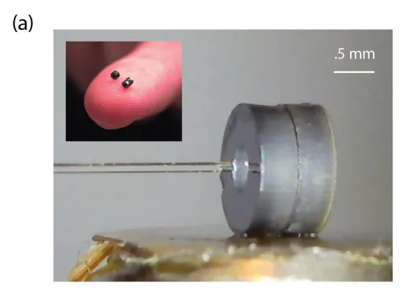
Beyond scaling quantum computing, the team is interested in the following applications:

Blind Quantum Computing

The concept of blind quantum computing (BQC) was proposed as early as 2001 (Childs, Secure assisted quantum computation, published in 2005). Its defining property is blindness: the server learns nothing about the computation it performs on behalf of the client.

Suppose:

• Alice possesses a valuable quantum state $\ket{\phi}$, a proprietary quantum algorithm $U$, and only limited quantum computation resources (e.g., some quantum memory and the ability to execute simple Pauli gates).
• Bob is willing to rent out access to his universal quantum computer.

A BQC protocol allows Bob to act as Alice’s delegate. Bob computes $U\ket{\phi}$ and returns the result to Alice, while learning nothing about either $U$ or $\ket{\phi}$.

The BFK protocol, proposed in 2008 (Universal blind quantum computation, published in 2009), removed any need for quantum memory or quantum gates on the client’s side: the client only prepares random single qubits, yet can have arbitrary quantum algorithms executed blindly. In 2016, Takeuchi et al. (Fault-tolerant verifiable blind quantum computing with logical state remote preparation) extended the BFK framework with stronger theoretical fault tolerance, which allows the server to execute longer gate sequences and tolerate higher levels of noise.

In 2025, Baranes et al. (Designing fault-tolerant blind quantum computation) designed an architecture that scales to fault tolerance while keeping the client’s requirements minimal:

• The client only needs the ability to measure server-sent photonic qubits in arbitrary bases (directions). The client does not need to store quantum states or perform quantum gates.
• The server needs a QPI: matter qubits are repeatedly coupled to photons, which are sent to the client for measurement.

This approach substantially reduces the cost of deploying BQC and broadens its market potential.

Super Long Baseline Interferometry for Astronomy

Quantum interconnects can be applied to astronomy. The basic idea is to exploit the nonlocal nature of quantum entanglement to (1) improve angular resolution by extending the baselines of astronomical interferometers, and (2) increase sensitivity by avoiding the need to physically transmit astronomical photons.

We first briefly introduce a few famous astronomical interferometer systems.

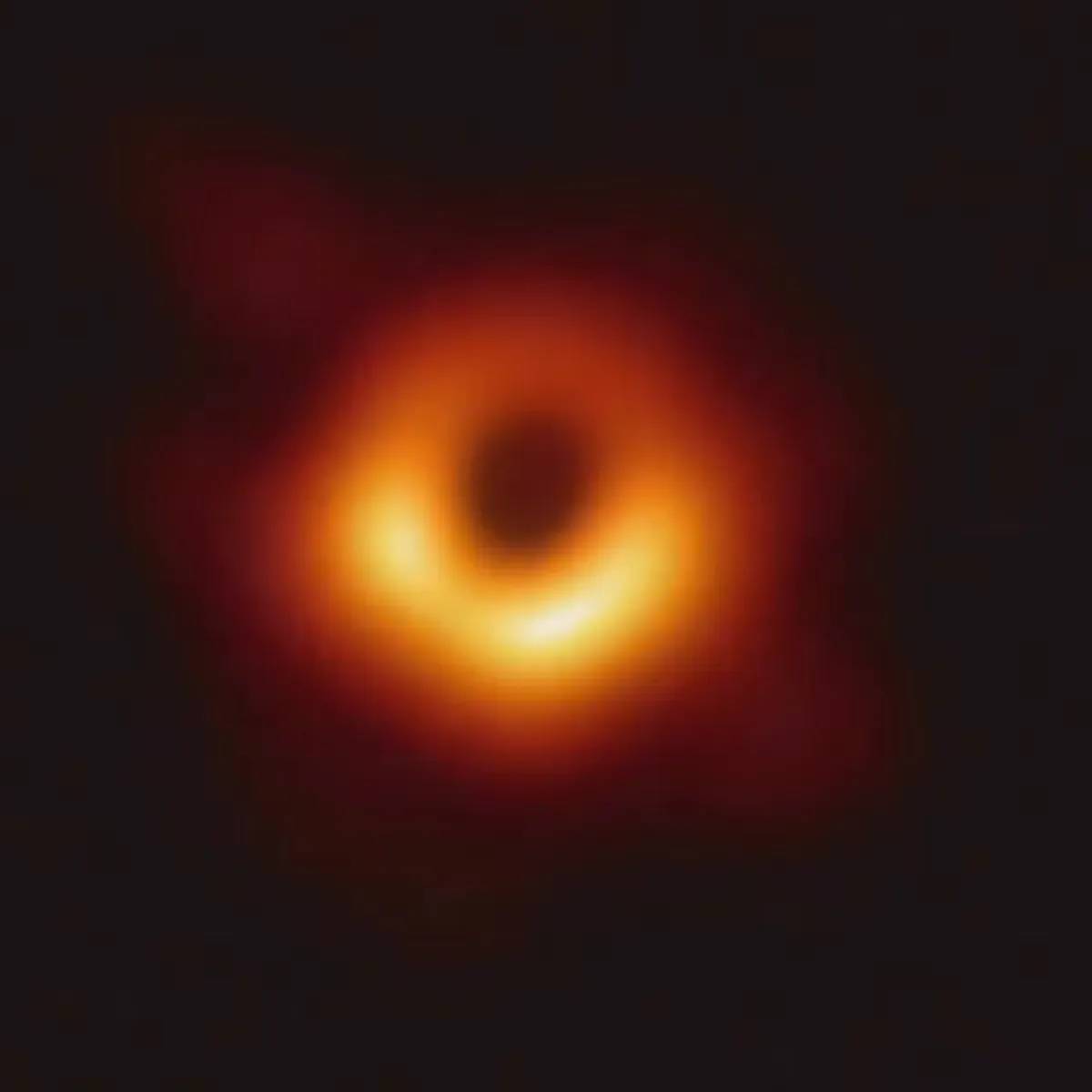
1. Event Horizon Telescope (EHT). Conceptual and experimental work began in the early 2000s. The project was formally launched in 2009 and reached operational maturity by 2017. The EHT uses a technique known as Very Long Baseline Interferometry (VLBI). Telescopes distributed across the globe are first synchronized using atomic clocks. These telescopes then observe the same distant astronomical source simultaneously and record phase information in electrical signals with extremely precise timing. These signals are then brought to a central correlator facility, where timing offsets are corrected and the signals are computationally combined to produce interference fringes, from which an image of the astronomical source can be reconstructed. The EHT produced the first direct image of a black hole. In April 2017, 8 radio observatories around the world observed the target simultaneously, collecting roughly 3.5 PB of data over about 40 hours. After nearly 2 years of data processing and analysis, the black hole image was released in April 2019. The EHT operates at a wavelength of about 1.3 mm (230 GHz), in the millimeter-wave radio band. Moving to still higher observing frequencies is difficult due to factors such as the stringent timing requirements exceeding the capability of atomic clocks, and atmospheric absorption by water vapor. The EHT achieves an angular resolution of about 20 microarcseconds in the radio band. This is equivalent to distinguishing a ping-pong ball on the surface of the Moon from Earth.

1. Navy Precision Optical Interferometer (NPOI). Completed in 1994, the NPOI is a Y-shaped array with three 250-meter arms. Its siderostats can be moved between piers along the arms to vary the baseline length for adjusting the angular resolution. Starlight collected at the stations is then transported in vacuum pipes. Adjustable optical delay lines are deployed along the pipes to compensate for differences in path lengths so that the extremely faint light collected by the stations arrives simultaneously at a central beam-combining facility to execute interference. NPOI’s maximum design baseline is about 437 meters, corresponding to a theoretical angular resolution of about 0.2–0.4 milliarcseconds. Unlike the EHT, which operates at millimeter wavelengths, the NPOI operates at 450–850 nm, covering the visible spectrum. For comparison, the Hubble Space Telescope has a visible-light angular resolution of about 50 milliarcseconds.
2. Center for High Angular Resolution Astronomy (CHARA). With first fringes in 1999 and its dedication in 2000, the CHARA array has a maximum baseline of 331 meters. It operates across visible and near-infrared wavelengths at about 500–2,500 nm, corresponding to angular resolutions of about 0.3–1.5 milliarcseconds, depending on wavelength. Like the NPOI, CHARA transports the faint starlight collected by its telescopes through vacuum pipes to a central beam-combining facility to execute interference. The array consists of 6 telescopes. Pairing the telescopes provides 15 distinct baselines.

Both NPOI and CHARA share a fundamental limitation: to improve angular resolution requires longer baselines, but that means transporting faint starlight over longer distances, which increases loss and phase fluctuations. Measuring the light separately at each station instead, as radio VLBI does with local oscillators, introduces vacuum noise from zero-point fluctuations, which is too much for faint starlight.

Is there a way to interfere the starlight captured at spatially separated observatories without physically transporting the starlight?

Yes, there is: by performing nonlocal interferometry.

The basic idea was proposed around 2011 by Gottesman et al. (Longer-Baseline Telescopes Using Quantum Repeaters). In the same year, Mankei Tsang (Quantum Nonlocality in Weak-Thermal-Light Interferometry) showed that in the weak-light regime, nonlocal approaches that measure the light from both stations jointly achieve strictly higher precision than local approaches that measure each station separately and then combine the results, such as the heterodyne detection used in radio VLBI.

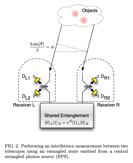
In 2025, Stas et al. (Entanglement assisted non-local optical interferometry in a quantum network) demonstrated nonlocal interferometry using weak laser pulses as stand-ins for starlight. The two stations were about 6 meters apart; spools of optical fiber extended the effective baseline to 1.55 km.

Their experimental procedure:

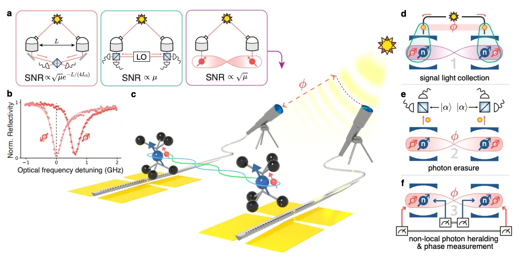
1. Each of the 2 stations is equipped with a quantum memory with 2 qubits: a memory qubit and a communication qubit. We denote the memory qubits by $m_1$ and $m_2$, and the communication qubits by $c_1$ and $c_2$.
2. The 2 stations prepare an entangled pair in the antisymmetric Bell state $(\ket{\uparrow\downarrow} - \ket{\downarrow\uparrow})/\sqrt{2}$ and store them in their memory qubits $(m_1,m_2)$, which provide a longer coherence time.
3. An astronomical photon may arrive at any time in a spatial superposition over the 2 stations.
4. When an astronomical photon arrives, with some probability it interacts with the communication qubit at each station, which writes its information into $c_1$ and $c_2$.
5. Interfere the astronomical photon on a beam splitter with a weak coherent pulse from a local oscillator, whose photon number is itself uncertain. This erases the possibility of telling which station the astronomical photon arrived at, which preserves its spatial superposition.
6. At each station, execute a CNOT gate over its qubits, with the memory qubit acting as the control. Recall that $(m_1,m_2)$ were prepared in an entangled state. If $c_1$ and $c_2$ contain information from the astronomical photon, that information has been transferred into the joint state of $(m_1,m_2)$.
7. Measure $c_1$ and $c_2$ (specifically their spin direction). In an even outcome (both spin up or both spin down), we know for sure that the astronomical photon was successfully captured by the system. In an odd outcome, the photon was not captured.
8. Conditioned on successful photon capture, the system is now in a state $(\ket{\downarrow_L \uparrow_R} - e^{\pm i \phi} \ket{\uparrow_L \downarrow_R})/\sqrt{2}$. The sign depends on the spin directions measured for $c_1$ and $c_2$. We are interested in $\phi$, the relative phase of the astronomical photon’s spatial superposition between the 2 stations.
9. Measure the above system state.
10. Repeat steps 2–9 many times to statistically estimate the value of $\phi$.

Given $\phi$ and system parameters such as the baseline length, we can infer the position of the astronomical source and reconstruct its image.

One can imagine a future network of nonlocal interferometric stations distributed across the globe. To achieve even longer baselines and avoid the atmospheric interference from water vapor, we could deploy the system on a network of satellites. Such systems would allow humanity to probe the mysteries of the starry sky in greater depth.